
This post really goes into the weeds, so only the technical experts should read the next sections which contains disturbing material that may not be suited for some audiences. The opinions expressed are those of the author and not necessarily the opinions of the website (which is actually the author’s) and are based largely on his ongoing re-reading of human history, still in progress. They are also based on numerous voyages to many hopeful prospects and working mines… including a few interventions on their behalf when things went wrong. The author even had a chance to participate in a couple of well-managed, developing vein mine projects where it was possible to recommend and execute appropriate sampling programs and grade control systems; the success of these ventures inspire me to make this post.[i]
Narrow Veins for the Post-Industrial Age
Geologists play an important and vital part at the bottom of the supply-chain pyramid of the build-out and we must re-double our efforts to identify value in heretofore chronically marginal mining districts and deposit styles to include narrow veins. A whole generation has gone soft from mining the last of the bonanzas and by depending on cheap energy and foreign capital to mine low-grade open pits where grade control doesn’t seem to matter, where maintaining reserve growth is just a pushback away. Now, a good number of us will have to re-focus on those messy, stubborn, and structurally complex deposits hosting those rare, but extremely “critical” minerals. A good deal of exotic metals and minerals occur in veins, or in discrete structural zones that can be treated as vein-like. Now, in 2026 (where did the time go?), we have some advantages that our less-equipped 20th century grand-geologists didn’t have. We have software packages that have tools for validating and exploring data, and for creating convenient, if not terribly accurate, vein and grade models. It’s “One giant leap for mankind” to borrow the somewhat awkward metaphor spoken by a highly suspect leaper on the moon. If we can estimate a credible and critical mineral vein resource, and our company is lucky (or connected), the Department of War will buy a big chunk of our shares.[ii]
Over the years and the experience with some narrow vein mines from epithermal and mesothermal environments on four continents, six U.S. states, and four Canadian provinces, and working with five software packages (now almost exclusively with Micromine), I have developed an estimation workflow applicable to narrow veins that is efficient and practical for mining requirements, within the limits of the quality of the underlying data. I’ll try to break it down enough here that it might be a useful guide for others.
Down to business. Isn’t posting great? No peer review, I get to approve comments, if any.
Considerations in Narrow Vein Modeling
Most narrow veins come with significant data quality problems. Data spacing and data orientation in these deposits that are mostly exploited by underground methods tend to be limited by various factors, including:
- Access availability, past and present, for drill platforms
- Insufficient budgets for new platforms
- Time required to do exploration work given the short attention spans of modern markets
In many cases, the data spacing and/or the data orientation with respect to the vein(s) available to the modeler are insufficient to robustly estimate the shapes, tonnage, and grade of better-paying areas (shoots). Readers can find some discussion of these topics by following the links to previous posts here: Drill Hole Spacing, Drill Hole Intersections, and Drill Hole Information Effect.
Data sets tend to have high coefficients of variation (CV); geostatistical methods such as kriging may have insufficient data support to be effective. If kriging is applied, it may produce overly smoothed estimates that are not suitable for mining at an economic cutoff. Any estimation method will tend to produce unreliable projections outward from the data grid. In partially exploited veins proximal to areas of tight data spacing, data clustering and issues caused by blended data types and multiple data campaigns tend to produce locally biased estimates. To a limited extent, data problems can be mitigated by way of EDA in the data preparation stage and by a reasonable estimation plan. Prudence often dictates a down-rating of mineral resource classification where data issues are known to exist.
A Test Case
To illustrate and compare results of different methods of estimation, I present a real-world example, comparing it to alternate and equivalent techniques which require more, or less effort. To protect the data source, coordinates are not provided and some place and commodity names have been changed.
The Mindout deposit, one of a number of such deposits in the Masskill District, is located in upper New York State near the shore of Lake America, approximately 20 km from the Niagara River crossing which, in 1813, was the site of one of the second series of U.S. invasions of Canada which began in the previous so-called Revolutionary War (Berton, 1980). The deposit consists of a vein swarm in Pre-American rocks of Grenville age hosting significant quantities of the critical mineral killingtonite (Ki) as well as several radioactive and potentially lethal byproducts. Killingtonite is used in conjunction with other critical minerals in the manufacture of chips used for drone navigation, triggers, motion controllers for directed energy applications such as inducement of Havana Syndrome and Lahaina urban renewal, in actuators for booby-trapped pagers, in weather modification, domestic air traffic control routers built in a small Middle East country, and in medical imaging and vaccine manufacturing industries, among other mostly peaceful applications.
Most of the deposit data are clustered chip samples; even the drill holes are clustered. A few drilling gaps are present on the flanks of the vein. In other words, a typical vein deposit data set.
Data Preparation
The starting point of a resource estimate is always a review of the database with special attention to items in the list below:
- Assay procedures and detection limits, lower and upper
- Metadata such as dates, companies, sample type and/or hole size
- Consistency and quality of sample location and/or downhole surveys
- Accuracy and consistency of data fields within, and between tables
- Understanding of the geological context and protocols for sample collection and measurement
- Bulk density measurements
Data originating from database software packages may be very clean. For example, in my experience most Acquire, Fusion, and Datashed managers have some good training; proficiency is gained by daily, focused use of the software. Database management and database development are somewhat distinct skills, but I think the need for the latter is less since software has evolved and improved. One of the cleanest databases I audited, though, was one built in-house by a geologist at the Fruta del Norte, Ecuador deposit with SQL It was a highly unusual blend of skills. And I did find another example of a very good home-grown database product nearby in the Silver Valley of Idaho. Most of us geos are data klutzes. We need to mess with the software enough to be able to direct the work, maintain quality, and apply tools for data analysis. We need database managers to support us and we need to appreciate their crucial role in advanced projects and operating mines.
Databases built in ACCESS, MXDeposit, Vulcan (ISIS), or in a workbook, rarely validate in my experience. The main weaknesses are in cross-table validation, but they also have weak or absent sample dispatch/sample receipt functions (exception MXDeposit). The latest versions of Micromine have excellent validation tools for imported databases that I always use for intra-table and cross-table checks before starting other EDA steps.
Graphic checks are next. We can plot the sample collars against topography or underground workings to see if any are up in the air, below the lake, or out in the wall-rock. Drill holes sometimes start at the surface and go upward to the sky because the sign convention of the dip in the database is different than the one used in our mining software. It must have been a geologist who came up with the idea of dip instead of just using “inclination” for everything, just to confuse a simple issue.
Once we have the drill holes going the right way, in the right township, and without any right-angle bends, and we have gotten rid of overlapping intervals, to’s less than “from’s”, samples that occur beyond the hole depth, repeated intervals, misplaced decimal points, and zero-length intervals, among other errors, we might wish to graphically check the coding in the key tables against geological model items.
Lithology might be important; certainly, we need some consistent coding that can be used to identify the footwall and hanging wall of each vein. Alphanumeric lithology codes are nice, but they are likely to be case-sensitive. If the logger is not constrained to pick a code from a property legend, there will be many different codes for the same rock which complicates analysis.
Do the vein wireframe surfaces snap to the corresponding intervals where data is intersected? That isn’t always the case. If they don’t it’s a stop sign and the issue probably needs to get fixed. What else? Have the database and vein models been reconciled with a backtag analysis to see to what degree samples codes match the wireframe codes or properties?
Missing Data Treatment
A few possibilities for handling missing data are given in the following cases:
- Drill hole crosses vein projection but there are no assays and no note in log
- Model a vein pinch-out at some fraction of the median data spacing or ½ the distance to the nearest datum, whichever is less, or
- Ignore if suggested by some other piece of information
- A structure is logged where vein projects; log is complete but no note of significant mineralization
- Model a vein pinch-out if there is confidence in the log, or
- If considered likely that no assay was obtained due to the interval being judged as low-grade, assign a very short width and a near-zero grade(s) to ensure that the divisor is much larger than the estimated accumulation
- Assays for one of the current economic metals are missing because only one metal was of interest in the past, and there are indications that the second metal is present
- Assign a low default grade knowing that it will underestimate grade
- Code blocks around the intercept and apply a filter to not estimate the blocks
Are pinch-outs, locations marked by holes which cross the vein projection but have no vein, handled in the database so that vein volume is not overestimated? Or does a vein “miss” reflect an offset, or a sharp orientation change, or a bad drill log, or an underground heading that accidentally veered off the vein? In the case of a “miss”, treating it as a pinch-out can produce very different local results than inserting a thin, dummy interval with zero grade. A geologist familiar with the data collection history and mine geology can resolve these tedious problems better than anyone else.
Does the last channel sample at the end of a drift mark the edge of the ore shoot or did world peace break out for a short time, tanking metals prices? Coincidentally, at this date, metals prices are tanking due to concerns about peace and a softening housing market. Or, maybe there’s more ore to get in that heading and the mine just shut down when it began losing money, or the government forced it to close due to war, or due to a tailings impoundment failure (latest one at this writing: October, 2026, Sombrerete, MX, List of major tailings dam failures). These minor glitches certainly have happened with a lot of gold mines and some critical minerals and may represent an opportunity for the next miner. [iii]
But I digress.
Drill Hole Intersections
We next want to understand sample widths and vein intersections. For chip-channel samples, how are they oriented relative to the veins? Were they taken as a horizontal width along a spray-painted line, or along the true width? Or, for a flat vein or seam, maybe across the vertical width? The Cantung Mine in Yukon Territories is an example where vertical channels were used for grade control when I visited in 1981.
Don’t assume the widths are recorded correctly. I worked with a mine in the U.S. where samples were taken along a horizontal line on an inclined vein but the sampler measured and recorded the true width instead!
Beware of underground or surface samples that do not sample a full cross-section; e.g., rib samples or raise samples where only a portion of the vein is exposed. You can’t use these for much.
Unless a drill hole trace is perpendicular to the plane of a vein, a correction factor is needed to convert drilled interval width to a true, horizontal, or vertical width. I encounter three ways that this is handled:
- Geologist records the angle of intersection of a vein contact in unoriented core angle (alpha)
- Using a jig for the purpose, both the alpha and beta angles of intersection of the vein contact are recorded on oriented core
- The angle of intersection is determined from the drill hole and wireframe triangle orientations at the point of intersection.
Method (1) only returns a valid correction to true/horizontal/vertical width if the drill hole is oriented perpendicular to the strike of the vein. I got slapped around pretty good in an audit a few decades ago for my ignorance of this fact.
Method (2) is robust and correct for the actual point of intersection. Roger Marjoribanks’s website (Roger Majoribanks) includes some great posts illustrating the method. The issue remains that there are always two contacts. What do you do? Average the results? If veins were planar structures, but they aren’t generally, any errors would be small. At least if the angle of intersection is very high; e.g., 60 degees or more, this latter statement is true. But if the drill hole intersects a contact at a low angle; e.g., 20 degrees, and the other at 40 degrees, the result of averaging is not going to inspire confidence. Did the hole deviate down the dip at the contact? Did a small-scale wiggle in the contact cause the big difference between footwall and hanging wall?
Method (3) addresses (or masks) the problem because the vein interpretation reflects an estimate of the average geometry of the vein at some scale using the cloud of proximal data points in its construction. In my opinion, it is best done using a medial reference surface between the footwall and hanging wall surfaces. Uncertainty remains with low-angle intersections. Notwithstanding, if the construction of the vein wireframe is done well, this method is acceptable. One can substitute the oriented core measurements where available.
Drill hole intersection angles should be considered in each of the following three study areas:
- Drill hole planning and execution – don’t plan holes that won’t intersect at <40 – 45 degrees because at less than this range correction factors are very significant. Also, a local wiggle in the vein may cause a planned 40 degree intersection to end up being a 25 degree intersection
- Vein modeling using samples, including drill holes – ignore and/or discount intersections <10 – 20 degrees and ensure that vein volumes influenced by such drill holes end up in Inferred classification, at best
- Grade estimates should not include drill holes with intersections <30 degrees, except, where in some cases, for estimation passes that are used only for Inferred resources
Don’t worry if up to this point you haven’t seen these rules of thumb. As QPs we are enjoined by our regulators to report how drilled width is related to true width, but there is nothing much else. When I explain my position on this topic, it generally makes sense to most geologists. It should be of utmost importance for narrow vein modeling.
Bulk Density
Bulk density measurements generally compose one of the least-populated tables in a sample database. It’s a bit odd considering that bulk density is one of the multipliers used to derive ore tonnage (see Dry Bulk Density). This situation amounts to an implicit assumption that there is little variation in a deposit, or that a few simple individual groupings can be averaged to reduce variance sufficiently. Imagine if we treated grade in such a cavalier manner!
Assuming one is not just dealing with a vein of quartz with scattered specks of free gold, it’s highly advisable to collect consistent, accurate, numerous, and spatially representative bulk density data from project stage through the mining stage. For narrow base metal and some other veins, it is generally possible to quantify the relationship between measured bulk densities and the concentration of one, or more, elements or logged minerals. Gangue mineralogy may also need consideration to develop a robust estimator of interval bulk density.
Accurate prediction of the bulk density of every assay interval may depend on the absolute concentrations of several metals which can serve as proxies for the vein mineralogy in the interval. Where more than one element or mineral is needed to obtain a robust correlation, multi-element interval assay data with methods like ICP are very useful. Bulk density measurements should be taken across the primary metal grade spectrum. However, many historical data sets don’t include a full suite of analyses. In Idaho’s Silver Valley, some mines just exploited silver-copper veins and didn’t bother assaying the lead veins for a decade or so, then switched back to mining silver in lead veins. And now, the mines are after antimony, or even gallium, and there is little historical data to be had for these elements.
Compositing
Reasonable options for compositing are:
- Equal-length composites that take into consideration assay length support, block and SMU size
- Full-vein composites of variable length
Option 1 is great but is not generally appropriate to narrow veins given wide data spacing and mining which almost always involves extracting across full vein width. Option 1 adds unnecessary apparent resolution not needed for likely mining scenarios. Option 2 is most appropriate, whether implemented via 2D or 3D methods. It is aligned with the selective mining units and sampling support in an actual operating scenario. However, sample support is not equal and merits evaluation for each vein; it should be addressed with an appropriate estimation method, the subject of this post.
If there is a clear dependence of bulk density on the metal or mineral content of a vein, and the relationship can be quantified using actual measurements, assays or logging information, then the bulk density of each assay interval should be incorporated with length as an additional weighting factor to derive composite grade (McKinstry, 1948, p. 48). This condition is clearly met for underground-mineable base metal deposits, or for deposits containing any other high-specific gravity metal in major concentration such as %Ki.
Metal-at-Risk
Some deposits should have some risky metal removed by capping, probably most of them. The major exception to that is for deleterious elements, where capping is generally considered to increase risk. Gold is generally a no-brainer for needing a cap threshold on assays or composites. Metal grades in base metals are not generally as skewed as precious metals and may thus have less risk metal represented in the database. A rule-of-thumb is that elements in major concentrations like percent are generally less skewed and present less risk mitigation through capping.
Before we start doing any fancy capping analysis, the first step should be a graphical review of possible ‘outliers’ in the data. If the high-grade samples are clustered spatially, they are not really outliers; thus, the most liberal threshold should be selected, the analysis re-run removing the “shoot” composites, or the analysis run based on domains, one of which contains the high-grade samples. If high-grade samples are scattered, the samples may be considered to be outliers based on statistical methods described below and subject to a cap.
If the estimation method used is a weighted grade estimate, one of the accumulation methods described in Estimation Plan below, the capping analysis should incorporate, at the minimum, length-weighting (i.e., horizontal, vertical, or true width). Depending on the importance of known mineralogy density control, length-density weighting should be the yardstick if there is a mathematical relationship between density and grade. This could be an equation generated by a multi-element regression of assay values or a stoichiometric one based on logged mineral abundances. For heavy minerals like Ki, this double-weighting is essential.
Inputs to capping analysis should also include declustering weights. These are best obtained by a carefully constrained nearest-neighbor estimate to a block model where the number of times each composite is used is written to a variable in the composite file. The blocks should be sufficiently small to ensure each composite gets a weight. Cell-declustering is an easy, but less robust shortcut. Thus, length, density and de-clustering weights should be considered in the capping analysis. The variable to cap in the case discussed here is likely to be %Ki_x_Width_x_Density_x_Declusterwt. This seems like a handful but that’s what the software is for—to make it easy. We are going to cap our composites back to the threshold suggested by our analysis; these are applied to the grade item which is then multiplied by the width item to obtain the Grade x Width estimation variable. This is the general case that can be simplified, if warranted; e.g., dropping the density or declustering weights. A minority of resource reports that I review consider any of the weights described here.
I recommend use of at least three evaluation tools for possible capping thresholds, such as:
- Histogram, generally log scale
- Probability plot
- Disintegration analysis
- Decile analysis
- Parker Risk-Hi simulation approach
The tools can be considered to compose two groups and it’s a good idea to use tools from each in any capping analysis. Histograms, probability plots, and disintegration analysis suggest outliers for capping based on data distribution assumptions and behavior, thus they have a broadly similar approach. The last two tools, a second group, choose cap thresholds based on the risk engendered by the relative metal content of each sample. There are a few other tools and rules-of-thumb that can be used, too, that I’ve skipped here.
With the popular probability plot, the process to pick an inflection point in the distribution tail gives a result that can vary from crystal-clear to a choice between several breaks. This is true to some extent with the histogram tail, or a disintegration plot as well. A decile analysis (Parrish, 1997) evaluates the risk associated with the metal content in each quantile of the distribution using empirical, experience-based rules. Dr. Harry Parker’s Risk-Hi program estimates the appropriate cap based on a declustered distribution of assays, an assumed production scenario, and a threshold of certainty in achieving production over quarterly and yearly periods.
In CRC’s experience, two or more approaches among the various tools and tool groups generally yield the same capping threshold giving some confidence to the exercise. For a feasibility case, or when there is great divergence in results, CRC recommends the Risk-Hi analysis as an arbiter.
Capping doesn’t fully address all the possible issues; a good knowledge of the deposit type, the deposit you are working on, and sampling factors should be applied to the capping procedure. For example, in some deposit types core assays tend to down-rate grade because of recovery or sample preparation. Canadian Archan greenstone-hosted nuggety veins sampled with split N- or B-size core tend to bias low for gold values while also returning high outliers. Nevada RC drill holes assays taken from below the water table can show extreme positive bias for precious metals. And what about dry RC from another era or a country that doesn’t have particulate dust suppression protocols in place? Maybe there’s some upgrading or downgrading going on in the drill hole? I don’t know… what did I do with my respirator anyway?
The geologist should also be alert to sloppy or inadequate sample prep and assay procedures by a company or lab, even fraud. It may color the choice of cap level. If there are biases or inaccuracies that can’t be addressed by capping, they should be integral to estimation of grade and/or to resource classification.
Backing up a bit, the first question I ask on the capping applied in a study is: “Did they cap assays or composites”? I have never understood the logic of capping assays unless a very high percentage of them are the same length. With composites we enter the realm of analyzing data in the context of a potential mining scenario. Of course, the geologist sampled a 20cm (minimum sample length for the project) veinlet with visible gold separately if nothing more than to understand the mineralization, but we know we will never design a 20cm-wide longhole stope, so who cares if the assay is spectacular? It will be diluted to a much lower grade if an economically meaningful interval is chosen. No, instead, let’s assess metal removal for composites for which the chosen length is related to bench height or minimum mining width.
Just because most software packages offer “hi-yield” search radius restrictions, a lot of geologists use this option. I have NEVER used this option. What is the basis for it? If metal-at-risk has been reduced with capping, why pile on with more restrictions on high-grade samples? Furthermore, I am not aware of an example of a QP assessing the separate impact of the high-yield search option on estimated deposit grade and metal. Conversely, we can simply add an uncapped variable in the estimation procedure which allows us to directly report the amount of metal removed from the block model and compare that to the prediction from the capping analysis.
Remember, our job isn’t to hammer the deposit by capping, it’s to identify risk metal if present, and quantify it. Any metal removed will be potential and should be known to the client.
Spatial Analysis
I wish there was more practical use for all the good and improving variogram software to evaluate trends in narrow veins. We can probably address the unequal support issue by calculating variograms with (true/horizontal/vertical) length-weighting, but we are likely to get unsatisfactorily short effective ranges. Blended data sets, high nuggets, and poor short-range definition due to wide drill spacing and the aforementioned factors contribute to non-robust variograms. We can try pairwise relative variograms, correlograms, or normal scores transforms to get something that might justify use for guiding or validating a search ellipsoid, classification distances, or an estimate using kriging. I define effective range as the range at 80% or 90% of the normalized sill of the variogram, relative variogram, or correlogram. In some cases, a first-pass search that uses the variogram with kriging can be fashioned from the spatial analysis. The advantages to this are significant in areas of clustered data.
I get ahead of myself. A good first step in evaluation of spatial trends and correlation is from the use of ID3 isotropic gridding, an old standby. One builds a point or block model parallel to, or within the vein wireframe. An estimate is done in 2d with the vein composites; e.g., KixT. We specify an isotropic and quadrant search for the first pass that ensures a cloud around much of the data, and a reasonable search distance and number of composites (6 – 10). We don’t want to impose our own bias on the trend. If there is anisotropy, that is, a preferential data trend, and there usually is one, it will show up in the grid which can be color-contoured in a section cut along the plane of the vein. We overlay the full vein composites color-coded to the grade or accumulation item(s) to be estimated to assess the pitch angle.
Implicit modeling tools found in various mining software can produce grade shells with little effort (and understanding). These are likely to show the general trends of grade and/or thickness. The NEW way is to use Micromine’s neural network algorithm that yields very insightful and relatively tight grade shells. The tool can estimate numerical or categorical items to a block model. The neural network results for KixHW and HW are shown for our test case (Figure 1) with no special constraints except for the specification of a decay-to-background distance:
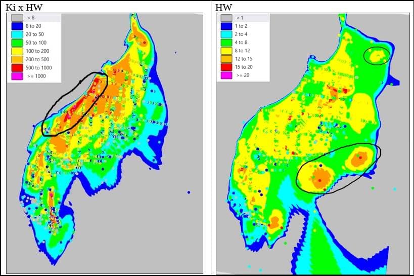
Figure 1 Grade shells estimated to block model with Grade Co-pilot (neural network) tool
At first glance, KixHW and HW show broadly similar trends. However, there are differences. KixHW shows more cohesion and continuity of high values along the left flank than HW. The HW trend is less pronounced, even discounting the impact of the choice of color legend for its display. HW shows a few areas of thickness on the right flank (circled) that don’t show up on the KixHW plot. For both variables, a prominent 45 degree pitch is evident, steepening at the bottom to near-vertical, suggesting the need for two orientation domains.
Local Anisotropy
We have a little problem with narrow veins—they aren’t simple planar features. Decades ago, this issue was routinely resolved by reducing vein estimates to 2D by flattening or unfolding, performing the estimate, and then transforming the block model back to real space. That was a bit of extra work, but the method was generally accepted and supported by some software packages. Nowadays we don’t like to do all that work so the major mining software packages have developed “local anisotropy” or “dynamic anisotropy” methods that rotate the search ellipsoid around corners to follow the local vein trend. This enhancement helps to ensure that samples within the maximum search distance are included in the estimation search neighborhood and that they are appropriately weighted. We can break the process for implementing local anisotropy into two parts:
- Determine the average pitch of mineralization within the vein
- Determine the local orientation of the vein in each block from the vein surface
In the first step, the pitch of mineralization determined using the average vein orientation will be rotated as necessary to match the local vein orientation determined in step 2, a separate procedure..
Step 1 Average Pitch
We will use each of the azimuth of the vein, its average plunge, and the pitch in a local anisotropy option for our estimate. In difference to the procedure for determining true/horizontal/vertical width from a drill hole intersection where it is evaluated based on two parameters, wireframe triangle azimuth and inclination (or dip), for our search ellipsoid we must define three parameters: azimuth, dip, and pitch.
To obtain orientation inputs, the following is a thumbnail of the Micromine interactive procedure. First, a plan projection and/or a series of clipped plans are drawn to determine the average azimuth of the vein. Next, a vertical cross-section projection and/or series of sections are cut perpendicular to the vein azimuth direction to choose an average dip. Finally, A sectional projection along the dip is cut to represent the plane of the vein. The latter gives a view looking toward, and perpendicular to the vein surface. The steps are illustrated in Figure 2 where the views are all clipped to simplify them and the far right image is the view perpendicular to the plane of the vein.

Figure 2 Interactive procedure for determination of azimuth, plunge and pitch of a vein with a grade shell contour as guide (blue lines); plan, cross-section, and projection along the plane of the vein.
With section clipping turned off, the ID3, implicit, or neural network shells created in earlier EDA steps are displayed with an identically colored composite sample overlay (not shown in Figure 2) for use in identifying the pitch direction. Pitch is recorded in different ways; in Micromine the process is interactive. In the estimation process, all three orientation parameters will be rotated to match the local changes in vein orientation in each block as calculated in Step 2.
Step 2 Local Block Orientation
The implementation of local anisotropy isn’t always perfect or appropriate. Triangle orientations can be assigned to each model block by nearest-neighbor methods to obtain acceptable results. As for the estimates of drill hole intersection angles, it’s best to use a medial reference surface to assign the block local orientations for control of the local rotation of the search ellipsoid. If solids are used, orientation anomalies will occur near the closed ends. A good check on the assignment of the local model orientation and predictor of the likely success of the method is to plot the assigned block model orientations in plan and section as plates or disks (Figure 3). The plates show that the orientations at the upper end of the domain are parallel to the closed end of the solid, which in this case might be the overburden surface. This is not a good result because the mineralization is in a steep vein.

Figure 3 Local block orientations determined from a domain solid (heavy black line) plotted as small plates; approximate location of alternative medial reference surface (green line).
If a reference surface is used instead of a closed solid, the local orientation problem shown in Figure 3 is avoided; block orientations will reflect the orientations of the vein walls.
If kinks in the vein are too tight, an unfolding technique which flattens both data and model to 2D might be necessary to ensure the right data are included in the search neighborhood.
In the case where a variogram for grade x thickness and/or width can be obtained that validates or supersedes the trends discovered by other EDA methods, it can be incorporated in an estimation plan with local anisotropy. Variogram weighting used in kriging is advantageous with clustered data when used within its effective range. The variogram axes will be rotated to the local triangle orientations in the block model just as is done for the search ellipsoid. If the variogram axis orientations are used to align the search ellipsoid, pitch will also be accounted for as long as the variogram calculation detects, and is aligned with the pitch.
Vein Block Models
Modern software packages; e.g., Vulcan, Datamine, Micromine, offer many options for estimation and replication of vein volumes in block models. These include:
- Sub-blocking to extremely small dimensions to provide volume accuracy at any scale;
- Choice of larger regular parent block size with a calculated % item;
- Variable block size in the cross-strike direction only
Option (1) tends to produce models of unmanageable size and block sizes that are inappropriate to the underlying data spacing. Users of a currently popular cult software generally must choose this option or choose regular blocks. Options (2) and (3) produce reasonably sized models and optionality for multi-vein block models. The other advantages of Options (2) and (3) are mine-wide block models that depict grade and tonnage synchronized to the selectivity of the mining method. The advantages of Option 3 over the first two are that the block boundaries visually lie within the vein boundaries and model size can be compressed several times over a regular model or a model “subblocked to extinction”, and blocks between veins can be removed. Most of the non-cult mining packages support such models, at least Vulcan, Datamine, and Micromine.
Some veins occur within a stockwork which may be thoroughly sampled and have significant, if generally much lower metal values. This was the case for the veins in the Kupol deposit, Chukotka. For this situation, halo wireframes were constructed. A modification of the block optimization included separate halo blocks and these were estimated separately. Between the halos there were no waste blocks retained. In this way, block model size was nicely constrained while still providing the necessary detail for development and stope planning. If the halo is not well-sampled it is better to figure out a default(s) value or just assign zero grade.
The following steps compose a condensed workflow in Micromine software to create the efficient and useful block framework for a steep-dipping narrow vein block model:
- Define a coordinate box to cover a swarm of veins
- Choose a fixed (small) parent block size for either X or Y, or X’ or Y’ (if rotated around Z), whichever is the strike direction, and Z block size just small enough to acceptably replicate the vein wireframe shapes and volumes
- Choose a parent block size for the other direction (X or Y, or X’or Y’), and a subblock size that will closely replicate the vein width at each location
- Create the blank vein model restricting blocks to wireframes (not possible in all software packages)
- Create a regular block model with the same definition except that in the width direction only one block is created that extends to the limits of the coordinate box; i.e., the block size in that direction is equal to the coordinate box size
- Add the two models together using the definition of the “large” block model—the new model has very wide blocks between veins and preserves the subblocked vein model blocks created in step 4
- Tag the model again with the vein swarm wireframes, deleting all untagged (waste) blocks
- At every X (or Y as the case may be), the strike direction, and every Z location, composite the vein subblocks to the full width of the vein.
Figure 4 shows an example of a model created in this way for a portion of the Kupol vein system.

Figure 4 A block model composited across a group of veins.
The block size is fixed in two directions and variable in the width direction.
Mining to blocks that are sub-blocked in all three dimensions (Option 1) is not practical. It’s a nightmare for the planner or geologist who wants to visualize what the grade is going to be at a specific location along the development on a particular level because there may be 1, 2, or more blocks across the vein width, each with different grades. The entire vein is going to be mined, thus this level of detail is unnecessary, even annoying and gives a misleading impression of accuracy. Block model sizes explode. If we composite across the width we can view the vein grades or thicknesses easily in either 2D or 3D.
Estimation Plan
Assuming that spatial analysis limits options and that the deposit in question has a high data variance, the estimation plan should be multi-pass with the first pass using close-spaced data and limited projection, hopefully guided by geostatistical spatial analysis results. This could be the basis for Measured Resources in the best case. A data cloud surrounding each block can be ensured by a quadrant search that requires data from at least three quadrants and 5 – 12 total composites, rule-of-thumb. The necessity for the minimum quadrant count can be explained by considering the common reality of dense sampling along sublevels with sparse drill holes between them. At least with a 3-quadrant requirement for a first estimation pass, the estimates for blocks positioned in the stopes between levels have a chance to include the nearest drill hole(s) instead of the search neighborhood being flooded with channel samples from a sublevel. It is not necessary to impose restrictions on the number of composites per drill hole because each provides only one composite per vein.
The second-pass search is enlarged, less anisotropic, is not a quadrant search, and retains restrictions on the minimum number of samples to include in the search ellipse. As a suggestion, second-pass sample minimums are set to >=2, maximum 6 – 8, but in some cases the thresholds can be set a bit higher. Data may all be arrayed on one side of a block, but that is preferable to forcing the search to draw on data a great distance away just to fill a quadrant.
The maximum search distance for each axis is selected based on the perceived anisotropy from trend analysis, and district experience. The second pass distances are generally a multiple of the first pass, and blocks estimated in the second pass as described here are going to receive a classification no higher than Indicated/Probable.
A good practice is to base the search radii, assuming they will be used as a basis for classification, on a range representing a percentage of a variogram/correlogram sill, or in an established district, on “customary”, experience-based distance criteria. In my opinion, it seems unjustified to base any search solely on the existing data spacing. That is circular logic if the sample data spacing was determined prior to geostatistical characterization of spatial continuity.
To what variable does this estimation plan pertain? In the attempt to answer this deceptively obvious question, let’s simplify the case and assume that there is no known relationship between assay value and bulk density. Given that, possible grade estimation variables written to a block model could be the following based on examples of machine methods with which I am familiar:
- Direct grade
- Direct grade, length-weighted
- Grade x thickness divided by modeled block thickness
- Grade x thickness divided by estimated thickness
- Grade x thickness divided by estimated thickness, use estimated thickness for tonnage
Method (1) is the simplest option. It ignores the support issue raised by unequal composite lengths. In effect, the modeler assumes that grade is entirely independent of vein width and that there is no correlation or dependence between them. The validity of the approach is questionable because grade is not demonstrably additive if support is not equal, nicely illustrated in the post by Cube Consulting (see References below), and in Bertoli et al. (2003). Another paper presents an alternative view of direct grade estimation (Marcotte and Boucher, 2002). Using the Walker Lake data set for its analysis, the authors conclude that if the correlation between grade and thickness is strongly positive, direct estimation of grade gives the best result. Conversely, a negative correlation gives the edge to indirect estimation and a zero correlation should return the same results. I really don’t understand how the discussion of Bias of the Indirect Method section in that paper applies to the way we implement accumulation method estimates. We don’t average ratios to get a block grade.
Nor, in my experience, is it common to see a general positive correlation between grade and thickness in narrow vein mines. Locally, we encounter positive correlations in those local areas which compose high-grade shoots. Shoots tend to occur where there is some structural complication and thickening in a vein, such as a vein intersection. McKinstry (1948) makes the observation that in some shoots grade trends with thickness, whereas in other parts of the vein there may be no obvious correlation. A more robust positive correlation coefficient between grade and thickness could be anticipated where the thickness of a layer of mineralization such as a massive sulfide has been deformed post-mineralization, as in the case described by Bertoli et al. (2003), but that deposit type is not the subject of this post.
The Mindout vein data set suggests that the relationship of grade to thickness can be more nuanced than just the check of the correlation coefficient suggested by Marcotte and Boucher. In a test vein for this post discussed below, vein width clusters within a range between 5 and 11 m (Figure 5). A discernible positive grade trend occurs within the lower half of that width band; beyond that wider intercepts appear to be lower grade. Whereas almost all the highest grades occur at vein widths <6 m with the highest outlier only 1.7 m wide.

Figure 5 Scattergram illustrating correlation of, and dependence on, grade with vein width
The near-zero correlation coefficient suggests the two variables might be independent, whereas the linear trend line suggests a negative dependency between grade and thickness. A linear fit is probably too simple to characterize the trend (s) across the entire range of widths. Even if we give the benefit of the doubt to Marcotte and Boucher’s conclusions, they do not touch on the difference between correlation and dependency. What sort of global and local accuracy do we obtain in the situation presented in the scattergram above if we directly estimate grade?
Method (2) is also extremely simple to implement in most mainstream software. Intuitively, it makes sense by giving wider intercepts more weight in the interpolation. It seems intuitive that Method (2) will more accurately estimate grade than Method (1) if there is some dependency on width. Method (2) is a shortcut which solves the support problem but it carries with it the implicit assumption that the grade and width trends and gradients are identical.
Method (4) is a more traditional approach involving separate estimates of grade x thickness and thickness, deriving grade by dividing the accumulation variable (G x T) by the estimated thickness, but it also has a shortcut form. The spatial trends and estimation plans for each variable should be evaluated and constructed independently, if warranted. In theory, Methods (2) and (4) should return the same result if the estimation plans for grade x thickness and thickness are the same in Method (4), probably a special case.
With Method (4), the estimated thickness at any point may be significantly different than the vein wireframe thickness modeled with other methods as illustrated in a white paper by AMC Consultants (Accumulation method). For example, conventional plan-section vein models, geostatistical methods, or implicit modeling might have been used to construct the veins creating an apples-to-oranges situation if compared to separate interpolation of grade-thickness and thickness. Thus, a “correct” grade in the block as derived from Method (4) might be applied to the “wrong” tonnage since the wireframe construction resulted in a block with a different width at each point.
Method (5) involves a coordinate transform through flattening or unfolding to a 2D environment for EDA and estimation. The vein walls can be constructed by positive and negative offsets of the transformed block centerpoints equal to ½ the estimated width. The blocks and points are back-transformed to the real coordinate system. Surfaces are constructed from the points and closed to make vein solids. This variant is well-suited to those cases where variography is practically useful and easier to calculate in 2D space. One should be cognizant of the possibility that the modeled vein may not snap to the composites depending on the method used to estimate width. Now, what do we with the vein we modeled initially with other methods, used for tagging at least some of the composites, and possibly for an unfolding? It’s not that convenient when your model does not exactly match your mapping and logging at every point.
A contoured difference plot on a VLP showing the differences between “geologically” modeled vein and estimated vein thickness for Method (4) will show areas that should be investigated. For example, where estimated thickness is very close to a sample point, the geology model is obviously the more reliable. The width estimate may be more valid between sample locations, and globally. If implicit modeling is used for the vein interpretation, the method can create improbably large volumes if not correctly constrained. These could possibly be corrected by creating control points for footwall and hanging wall from the block direct-estimated widths at enough locations to constrain a re-run of the geology vein interpretation. Depending on the magnitude of the differences seen globally and locally, and the stage of the project, the 2D variant of Method (4) might be very acceptable instead. It is decidedly more robust in some respects than the 3D methods.
Method (3) is quick and easy and should be comparable to Method (4) if, as is unlikely, the wireframe was constructed based on a similar estimation plan. Given a very good data pattern and perfect alignment of model blocks to a uniform vein strike, this extreme shortcut might yield comparable results to the other accumulation methods. With Method (3), one should be careful to use horizontal thickness unless the block model construction included a second rotation into the plane of the vein—not common.
In summary, Method (2) and (4) have the major advantage over Method (1) of eliminating the important data support defect of the latter method. Method (2) is exactly equivalent to Method (4) under a certain condition discussed above, otherwise it should produce somewhat different results that will be hard to analyze. Method (3) derives grade from two different thickness values, and tonnage from the geology wireframe. Implied tonnages from Methods (1), (2), and (3) are not likely to yield the same implied tonnages as the wireframe-based tonnage. The Method (5) 2D variant is the most robust and internally consistent model but is unlikely to exactly match reality at sampling points.
In our test case, below, the wireframe was constructed using implicit methods and can’t be expected to yield near-identical results to a wireframe constructed based on a geostatistical method. The estimation plan for width is the same for Methods (2) and (4) to facilitate comparisons of results between them. Method (5) is our “base case” to which the best shortcut (Method 4) is compared.
Test Case Results
A blank model framework is constructed comprising blocks sub-celled along the direction perpendicular to the vein strike with small, fixed block sizes in the other dimensions. Model rotation is around the Z axis to match the average vein strike . The sub-celled blocks are then composited across strike within the vein to create a single block at any particular level along the vein strike, the workflow described in the section Vein Block Models. In effect, each block estimate will represent a full vein face composite grade across the horizontal vein width, or better, a full round (or multiple of a round) grade if the extraction is to be by drift development.
The estimation plan is identical for the four methods except for the killingtonite input variable which may be direct or indirect. And in the case of the indirect methods (3) and (4), an extra calculation is made to derive the grade in %Ki from the horizontal width (HW) variables.
The vein composites are plotted on a vertical longitudinal projection (VLP) of the vein wireframe; i.e., the vein footprint. Figure 6 shows the grade estimation results of Methods (1) – (4) across the full vein horizontal width at an 8% Ki cutoff:
Figure 6 VLPs showing results for Ki at 8% Ki COG using different methods, from upper left to lower right, Methods (1), (2), (3), and (4).
At first glance, all the estimates yield similar results. They all capture low and high-grade areas, and all have polygonal-looking grade contours in areas of low data density at the peripheries. Each method captures the general mineralization trend, a pitch to the left in the upper and central areas, steepening to near-vertical in the lower part of the vein. It’s apparent that the effects of the different estimations are visually incremental; however, the direct estimate of grade does appear to form larger and higher-grade shapes on the periphery.
The +8% Ki comparison shown in the VLPs is summarized in Table 1:
Table 1 Grade-metal comparison to accumulation method to three alternative methods using full data set (8% Ki cut-off grade)

The more densely drilled area represented by the M&I classification show modest variances to Method (4), except for Method (3) which returns lower grade than Methods (1) and (2). Direct estimation of %Ki (Method 1) is biased high compared to accumulation with respect to tons and metal in all categories, but especially in the Inferred blocks where the variance to other methods is large. The direct estimate with the length weights (Method 2) yields an exact comparison to Method (4) but this is expected because the estimation plans for G x T and T are the same in the test case. The most robust shortcut, Method (4), reconciles well in the M&I category to the most robust method, Method (5). The result may be due to the large amount of data and/or a well-constrained and appropriate algorithm used to construct the vein wireframe such that its volume matches the horizontal width estimate. Vein tonnage reconciles well in the Method (4) Inferred category but grade shows a low bias compared to Method (5).
Discussion
A longstanding consensus is that accumulation methods are the most defensible and robust for estimating narrow vein tons and grade. The accumulation methods involving (Grade x Thickness)/Thickness to extract a grade, whether 2D or 3D, avoid data support and additivity issues. They are not necessarily aligned with the entire estimation scheme, however. If, as is often the case, wireframes are built using conventional plan and section interpretations, or a numerical modeling method different than that used for the T-G-M estimation, the estimated width divisor may not equal the wireframe width at actual data points. The potential width discrepancies are potential pitfalls in any of the narrow vein methods described here. It’s worth recognizing, and if time permits, evaluating this for every estimate done by accumulation. For example, one could evaluate discrepant areas of a vein with a difference plot (Wireframe horizontal thickness – estimated thickness) and possibly adjust either the estimate or the constraining vein wireframe to reduce their size and magnitude.
The robustness of each method depends on several factors:
- CV of the data and quality; data types, data spacing, data history
- Correlation of thickness and grade—negative, absent, positive?
- Degree of dependence of thickness and grade—there tends to be some
- Do thickness and grade have the same trend directions—if not, estimation plans should theoretically be different; practically this can cause issues of model fill and grade anomalies in open data grids
- If thickness and grade trends are the same, do they have the same gradient; e.g., may need to use ID2 on thickness and ID3 on grade-thickness?
- Inaccuracy or bias in the wireframing exercise, if done as a separate exercise
- Does the vein have hard breaks such as cross-faults or host rock changes, and are they modeled for use as constraints?
- Does the estimation plan provide for a degree of declustering and for a data cloud around each block?
The accumulation methods described above involve a considerable amount of analysis and many steps to implement thoroughly and appropriately. In my experience, I have reviewed many estimates that use the same estimation plan for grade and width, and in polymetallic veins, for different metals. For example, a silver estimate may just piggy-back on the build-up and implementation of the gold estimate plan. Especially for properties with several, or even dozens of veins, the time and/or experience needed to produce reasonable models isn’t always available; most estimates employ various shortcuts, whether implicit or explicit.
The Method (2) “shortcut”, direct estimate of grade incorporating length (thickness) and density weighting as described in this post is comparable to the 3D accumulation method under certain conditions. It avoids data support and variable additivity issues. If grade X thickness and thickness both exhibit the same trends and gradients, Method (2) should return the same results as Method 4, as demonstrated in Figure 6 and Table 1 . Otherwise, it is indeed a shortcut compared to a Method (4) estimation with distinct grade and thickness estimation plans . In my somewhat limited research on this and from my own experience, Method (2) is not in common use, in part because of inflexible options in some of the mining software packages; e.g., the cult software. However, my own experience with it is generally good provided the drilling grid is reasonable and the grade and thickness trends are similar.
Direct estimate of a grade variable using variable width composites (Method 1) is the ultimate shortcut and our test case tends to confirm the consensus view that accumulation methods are preferred. It violates the assumption of equal data support which renders grade non-additive. Prior to selecting this method, one should be able to demonstrate that the grade-width correlation is zero and that there is no dependency of grade on thickness. We saw in the test case discussed here where peripheral areas of the vein have a high bias compared to accumulation methods and across-the-board it has the worst comparison to the other methods tested. I suspect that one must be lucky for this method to produce good results.
One other method not discussed so far in this post is a true 3-D estimation method using fixed-length composites. I have attempted this in the past and have reviewed a few such models. This writer believes such an approach is generally impractical for a narrow vein; i.e., one for which the potentially economic parts average just a few meters in width. As a side-benefit, the method creates huge block models with multiple blocks across the width of the vein. No one wants to see these again unless loading huge block models to memory provides extra-long paid coffee breaks. It has a place in veins wide enough to be able to make a U-turn in a heading with a Toyota Hi-Lux pickup such as in the Big Bend ore shoot at Kupol, Chukotka, or this one:

All accumulation methods applied to the Mindout vein test case, except for the extreme accumulation shortcut of using grade x horizontal width and wireframe-defined block horizontal width (Method 3) as a substitute for a separate thickness estimate, seem to return results for grade and metal in acceptable ranges in areas of good drilling density and spacing.
I have glossed over the importance of data and drilling quality apart from the brief bullet list above. This recalls the Harry Parker adage: “In general, an ounce of geology is worth a pound of geostatistics; this may be disappointing to geostatisticians with no geological background; tough”.
Validation and Classification
This post is getting very long, but it would be remiss to completely skip over two essential parts of an estimate, validation and classification. The principles for these aspects of a mineral resource estimate are the same as for any estimate to which notes should be made of additional checkpoints.
For validation, I recommend the following steps:
- Graphic review in VLP of the results for each variable estimated compared to the data support
- Check the estimation parameters and estimation audit report statistics for each element, each domain and each pass (Micromine)
- Prepare a global bias table comparing the nearest-neighbor estimate to the interpolated final at a zero cut-off grade
- Plots swaths in each dimension comparing the estimator to the nearest-neighbor result and the weighted composites
- Prepare a table comparing the amount of metal removed by capping using the capped metal variables vs. the raw metal variable
- As deemed appropriate, re-run any of the above checks after pre-classification of the mineral resources, focusing on the critical Measured+Indicated categories
- Assess the impact of any discrepancy between the geological model and estimated widths with difference plots
- Reconcile depleted areas to production data, as available
- Compare the resource to the previous one
While nine (9) steps are suggested, several can be generated and scripted by statistical and reporting tools embedded in the mining software package which decreases the time spent compared to the old days. The last two steps may involve some adjustments, re-runs, and in the case of reconciliation, hair-pulling.
The simple term “classification” is not adequate to describe what really is a two-step process. First, we assign what, in effect, is a pre-classification based on estimation confidence criteria. These include sample distance, pass, and/or number of samples, etc., whatever the QP feels constitutes an estimate with appropriate confidence for the pre-class category. But then our regulators in various jurisdictions require that resources in each category have “reasonable prospects for eventual economic extraction”. That requires an overlay of some sort of economic test like the calculation of an optimized pit based on various recoveries, costs, and metals prices, etc., or for an underground mine, something similar such as a stope optimization. Anything inside the resulting shapes can have a classification of Measured, Indicated, or Inferred. Anything outside is just potential. I am very much in favor of applying optimistic prices for metals resources while maintaining much more conservative ones for reserves.
Geologists are generally concerned with “pre-classification” even though I made up the term. A geologist can generate an optimized pit or a general underground mine perimeter as a proxy for a mine plan to report classified mineral resources, but this is often delegated to a mining engineer. Mining engineers are qualified to report mineral reserves.
A Micromine workflow comprises the following steps for mineral classification in narrow veins:
- Identify the pre-classification confidence criteria for each category to be used to assign Measured/Indicated/Inferred categories to each block based on estimation results; e.g., nearest or average distances to samples, pass number, number of samples, etc.
- Viewing the vein in VLP, plot blocks color-coded by each of the three pre-class categories 1,2,3
- Create outer grade shells for each category; the Inferred one encloses pre-class codes 1, 2, and 3, the Indicated one encloses pre-class codes 1 and 2, etc.
- Create a silhouette perimeter string (2) around each shell sequentially starting with Inferred, in the process removing inlier strings, and small, isolated strings—check for closure and any clean-up needed
- Use a smoothing function such as a point-honoring spline to smooth each class perimeter string
- Extrude the class strings to class solids far enough in front and back of the vein footprint to cover the block model—validate these “cookie-cutter” solids
- Assign a new class code variable values of 1, 2, or 3 in each block in reverse order in a tagging operation using the class shells
- Assign a depletion code and/or percentage to each mined (or sterilized) block to enable reporting of remaining resources
Thus, confidence criteria are applied assign a pre-class code, then several smoothing steps are used to produce contiguous groups of blocks with the same classification to avoid the “spotted dog” effect (Stephenson et al., 2006). The above procedure can be largely scripted with pauses to manually edit the intermediate products. Step 8 may involve a set of solids for mined-out material and another for material deemed inaccessible or unmineable. As with most of the Western world’s standards and regulatory guidance, it’s the Wild West with much discretion left to the CP or QP.
Flashback
In the 1970s and 1980s I made long sections and computed resources on them using polygon methods. McKinstry, (1948, p. 59-60) describes a couple of common methods that I recall: 1)Polygons based on projections of half the distance to the neighboring data point; or 2) Triangular method. For grade, the product of length with width and area (L x W x A) for each sample string was calculated, then the average grade of a block was determined from (∑L x W x A)/(∑ L x W). Tonnage was calculated by determining the volume from the area of the polygon and the average width of the strings ∑(L x W)/∑L, multiplying the result by a bulk density (or dividing by a tonnage factor).
The introduction of electronic plotters made it easier to print out drill hole VLPs instead of having to draft them on a linen or mylar by hand. We plotted our sample data and drew polygons by pencil or with a rapidograph pen around each chip-channel string or drill hole. We had rules for projection distances; e.g., half the distance to nearest sample string or drill hole. We kept our calculations for each polygon in hand-written notebooks. We capped grades based on customized or standardized rules from the district, mine, or the deposit type based on experience. High-grade areas were confined to separate polygons—equivalent to domaining. The VLPs for each vein were stored in hanging files or large map drawers. I piled my paper section updates on top of hand-drawn linen ones from the previous generation. I don’t have a steady-enough hand or good enough vision to build one of these now. It’s a lost art; those sections and the plans which supported them can be destroyed by fire but not by an EMP burst or a server accident.
Polygonal methods have been found wanting for concerns of bias, particularly conditional bias, and the overriding concern with the labor involved to produce them. They are largely superseded by numerical methods, perhaps to a degree that is not justified. A hand-drawn, measured, and calculated polygonal resource required a great deal of local knowledge of the orebody. Sure, there could be bias and inappropriate projection of high-grade material. Was that any worse than what we can do with our convenient software? I think the main advantage of our computer methods is the ability to support a high rate of production with a smaller, and thus less expensive technical staff, although the latter issue could be offset by slashing executive salaries and perks and hiring and training more staff at the operations.[iv]
New Geological Order
At the end of the day, there is still some art applied to the science, but let’s at least get the basic arithmetic right and use good sense. The best chance to create a good block model is for the geologist to have a good deal of experience in the deposit through drilling it, understanding the production requirements, as well as hands-on sampling and mapping. There is no place for a job description at a mine such as: “Resource Geologist”. Resource estimation should be a shared task within a project or mine geology team. Training in traditional estimation methods and geostatistics should be provided in schools and/or by the company, starting with a basic course and continued by knowledge transfer from senior to more junior staff. Resource modeling in the narrow vein setting is quite challenging and requires a blend of skills and experience. Routine outsourcing to consultants represents a commitment to mediocrity.
The staff should apply common sense and geostatistical tools and principles to the estimation of grade and tonnage. It shouldn’t rely 100% on packaged software to dictate a workflow, rather, the software must support the project’s needs or be discarded for another more suited to the tasks. A smart mine geologist will continually ask for, and a clever mine geologist will get to drill more holes than those provided by the exploration phase. I have yet to visit an over-drilled deposit. At the risk of misquoting myself, I think we drilled out the Cannon Mine stopes on 15 x 25-foot centers. It was a rational spacing established before I arrived halfway through the mine life. We made money with gold as low as $300 and the seven stages of a project were largely avoided…

Nobody complained. The ore was mostly where we said it was. Reliable mine plans could be made with the models. We met our production targets in a tough price environment.
I wish to thank my past mentors for their tutelage, and above all, patience. Best of luck to all of you in the trenches.
References
Bertoli et al. 2003; Two-Dimensional Geostatistical Methods — Theory, Practice and a Case Study from the 1A Shoot Nickel Deposit, Leinster, Western Australia; 5th International Mining Geology Conference; p. 1-7.
Berton, P., 1980; The Invasion of Canada, McClelland and Steware, Ltd,, 363 p.
Cube Consulting, Two Dimension (2D) Estimation and Application of Accumulations.pdf; Cube Consulting Website
Discovery@Illinois, Correlated, Uncorrelated, and Independent Random Variables, Data Science Guides; Website
Dominy, S. and Camm, G.S., 1999; Resource Evaluation of Narrow Gold-Bearing Veins: Problems and Methods of Grade Estimation; Trans. Instn Min. Metall., 108, January-April, 1999.
Marcotte and Boucher, 2002; The Estimation of Mineralized Veins: A Comparative Study of Direct and Indirect Approaches; Explor. Mining Geol., Vol. 10, No. 3, pp. 235–242.
McKinstry, H.E., 1948; Mining Geology; 680 p.
Parker, H.M., 1996, Grade Capping; pers. commun./unpublished MRDI report
Parrish, I. 1997, Geologist’s Gordia Knot: To Cut or Not to Cut; Mining Eng., April 1997
Webster, R., Narrow-vein Modelling and Mineral Resource Estimation; AMC Consultants Website
End Notes
[i] Of course, the overriding goal of this post is to help our government obtain the critical minerals (and, er…metals) we, and, well…IT needs to be able to surveil, control, and, if necessary, blow-up people and things. This is where narrow veins have an important role to play, as we shall see. If you can get through the next section, you have what it takes to propel us forward. Make (whatever) Great Again! Add your own Barnum statement …
—————————————————————————————————————————
[ii] Much has changed in the last few years because of the headlong race to (extinguish a large percentage of humans) build data centers to support the greatest grift to mankind—Artificial General Intelligence, aka A.I. A.I. is changing the way we live our daily lives. Soon we will no longer need to read, write, or bother with boring research and problem-solving. Instead of sending our golden youth to fight wars in the trenches, they will be able to create great havoc and destruction on Oceania’s “enemy”, Eastasia, from secure, if possibly a bit damp and drafty, underground bunkers with help from their A.I. assistants. All our basic needs will be determined by algorithms and will be met according to our ranking in the social scoring framework, it, of course, being calculated by A.I. You won’t even need to read the post. Your A.I. agent will be able to give you an oral summary in a pleasant voice that sounds like your old childhood robot nanny. Or maybe give you a scolding: “Luddite is not a critical mineral, Winston.”
—————————————————————————————————————————————————
[iii] The government subsidized production of copper, lead, and zinc from 1942 to at least 1945 by guaranteeing prices at higher-than-prewar levels, while closing gold mines to force labor to shift to base metal mines. Bradley Mining Company got government support to operate a marginal deposit of antimony in Idaho during the war, eventually supplying 90% of domestic production. The government also gave technical support during the mid-century wars to producers of tungsten, tantalum, graphite, quartz, and other minerals. The DMA, and later DMEA program of loans and subsidies for exploration was created around the outbreak of the Korean War (1950) and then limped along to its final death in 1974. When all these government programs ended many projects shut down leaving empty towns and lots of pollution.
At least in the case of Bradley’s mess, Dolly Varden trout are (were) found in the old Yellow Pine pit traversed by the South Fork of the Salmon River despite all the deadly potential pollution. That was the case a couple of decades ago in my work with Hecla which owned a big chunk of the claims there. I hope the fishies survive the new operation.
All that history kind of reminds me of what’s going on now in 2026—direct government investment in companies with projects under a whole bunch of 3-letter agencies. Ones like Lithium America’s Thacker Pass: more than three years into construction and the latest news is a $0.9 billion cost over-run on a capital budget finalized just 18 months ago, a 30% bust—no worries, just draw down more of the $2.23 billion USDOE loan. Besides the U.S. taxpayer, probably the 2nd biggest sucker is GM which owns about 38% of this gem. I guess in 2021 it looked like a good investment.

More recently, July 24,2026

Now, fewer people want a lithium-powered electric car that can suddenly burst into flames. I wonder how this will work out for GM?
And for antimony, Perpetua Resources’s re-named Stibnite Gold Project finally gets off the ground, but only after receiving a $2.9 billion loan from the U.S. EXIM. It’s really a refractory gold mine containing a lot of arsenic and with a shaky antimony resource. Its heyday was well back in the last century, supported at times by those wartime government subsidies. It turns out that only about 15% of antimony production goes into war-critical bullets, much of the rest is used for fire suppression. But warfare is now dronefare; drones, not bullets are the new weapons of war. Well, at least us taxpayers will help get some gold out of the thing. Or will we?

Source: /investornews.com
Since the beginning of 2026, antimony climbed in price and is currently dropping steeply in price. So is gold. Just in time for a new mine to open.
And rare earths are not forgotten by our government because according to the U.S. Department of War wbsite (Rare Earths) : “The Chinese Communist Party has implemented aggressive actions to endanger the global critical minerals supply chain and ultimately undermine American economic and national security”. Those pesky Chinese! Was that text maybe written by the hormone-boosted, tatooed current Secretary of War? To help counter that “threat”, MP Materials just got a $150 million loan to improve its Mountain Pass, CA plant. It was all part of the One Big Beautiful Bill Act of 2025.
MP Materials net losses narrowed somewhat in Q3 2026. How many times does this mine have to fail before it finally closes?
Talon Metals gets a $20.6 million matching handout for exploration expenses to find some more nickel Nobody ever offered that kind of money to any company I worked for, much less me. There are other government ventures in scandium, boron, and who-knows-what-else? I guess taxpayers are looking to invest (give away) up to $100 billion eventually.
Doesn’t look good for world peace, does it? Or balancing the budget.
————————————————————————————————————————-
[iv] And anyway, there were screw-ups with the old ways. A one-time major mining company ASARCO, now just a part of Grupo Mexico, ran a certain vein mine from 1976 – 1995. All the reserves were calculated by polygonal methods on vein VLPs per the convention at the time. Tonnage was calculated as the long-section Area X True vein width from the sample strings, and a tonnage factor. The trouble with that is that the veins in the mine generally dip ~60 – 70 degrees. ASARCO geologists should have used horizontal width instead of true width for calculations on a vertical projection. Thus, for at least 20 years, and maybe longer, all ASARCO’s resources/reserves were reported with an error of ~ (-)10-15% for tons and metal (not grade). I made this forensic discovery about ten years ago when I was helping the mine transition from manual methods to computer-assisted resource estimates. One could charitably call the calculation error a “geology call factor”. So, who says the old-timers were great? Ok, the guys who wrote the books and articles 80-130 years ago that we still find valuable were great. The rest were just like us regular geos, the 95% of us.