I’d like to introduce the patient reader and my clients to a conceptually simple tool that is useful for the assessment of resource risk. The Drill Hole Information Effect (DIE), as I propose to call it, is the observation that the deeper portions of a mineral resource are generally estimated with less sample information than the upper portions. This engenders resource risk.
Grade control doesn’t seem to be too interesting to the mining community these days, my take on it anyway, and now we have the “Green Distraction” with which to contend. We would need to produce lithium at 2019 levels for 9,000 years (Michaux, 2021) just to replace one generation of current fossil fuel units. Up against the ESG crowd, I just don’t know how to even start a conversation and I’m done with the latter on this blog for now. Let’s try something else–DIE!
Having by now read many dozens of the now-standard NI 43-101-format technical reports on properties, sometimes just for fun, other times for amusement, and still others for professional enrichment, I have concluded that sample spacing, most commonly drill, or hole spacing, is poorly quantified in almost all of them. We find statements like: “In 2015, an infill drill program was undertaken on a 100 m x 100 m grid.” That was the plan, what was the actual? If the holes were inclined and drilled along a variety of azimuths and inclinations, how was the spacing measured? In an earlier post, What’s the drill hole spacing for your project?, a rigorous 2D method is briefly described for measuring and displaying drill spacing through a deposit by bench using bench composites, or on a longitudinal section using vein composites. A graph included in that post shows a dramatic increase in drill spacing below a certain bench. In my 20 years of experience applying the Hole Spacer 2D workflow, I have yet to find a resource that has a completely uniform drill spacing from one level, or one area to the next.
The output from Hole Spacer 2D for the set of levels or benches that you want to evaluate, or from another tool you may have for the same purpose, provides the data needed to evaluate DIE. There is a question of whether it is most appropriate to use the mean or the median as the central measure for drill spacing. I generally prefer to plot both, but I almost always express the drill spacing with the median values. Because we over-drill the center of a deposit and under-drill the margins, the mean drill spacing curves tend to plot at higher values, receiving undue weight from the deposit fringes.
Once we run a hole spacing analysis, I always advise a final graphic review of the benches or long section with the spacing results in hand to assess potential impact on a mineral resource.
One of the outputs I track with the Hole Spacer 2D output is the simple average metal grade(s) per bench. If the metal grade of the deposit increases with depth and distance from your rock hammer, resource risk is increased. Note that this is the case seen in the graph of a real (big) deposit in a country that locked down all its inhabitants hard for over a year for absolutely no reason at all except maybe to stop their massive protests, and where the water circles the bowl clockwise, in theory, and for which multiple companies have tabled several feasibility studies and it still is not in production, thankfully (I’ll die with the knowledge of the secret location):
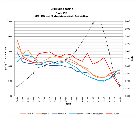
The graph shows that even as drill hole spacing increases, the grade also does so moderately. Thus, drill hole information effect (DIE) risk is a combination of drill spacing and metal grade suggesting the following relation:

,
The DIE factor is the product of the change in drill spacing at the top and bottom of the deposit composing the Drilling Information Factor (DIF), and another factor which compares the grade over the same interval, the Grade Factor (GF). The calculation of the factors is broken out in the simple equation below:
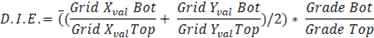
where, Grid values are entered as spacings in meters or feet, as explained below, and Grade in the metal grade units. The equation calculates factors for each grid axis from the values entered and then averages the result to give the approximate result for the drill grid spacing factor. For example, if Grid Top in X and Y is 50 m x 50 m and Grid Bot is 100 m x 50 m, then the equation will return ‘1.5’. The result is in this case intuitively exact because it takes four holes to make the bottom grid cell and two additional holes to fill it in for the top drill grid, or 6 / 4 = 1.5. Likewise, if Grid Top X and Y dimensions are 50 m x 50 m and Grid Bot is 100 x 100 m, then we should enter ‘2’. The fit isn’t exact because it will take nine holes to compose the infilled grid compared to four holes to compose the 100 m x 100 m grid, a factor of 9 / 4 = 2.25. Rounded, this can be considered ‘2’.
Implicit in the equation is the assumption that these factors are multiplicative and not additive, admittedly an arbitrary choice. This assumption does allow for some interaction in the two component factors of DIE, whereby one factor can either minimize or amplify the result, depending on the case, and we can conveniently set an ideal benchmark value for DIE as ‘1.0’. For this ideal case, spacing is equal from top to bottom and there is no grade trend. A large DIE factor can be caused by the opposite, and quite common case, where the drill holes spread out at depth and probe the high-grade feeder zone. For this type of deposit and drilling program, the DIE acronym has special meaning when thought of in the context of the probability of the project’s success.
No introduction of a new concept is complete without a few real case histories, names changed to protect confidentiality. Case 1a, a dog’s breakfast grid of shallow holes by early operators filled in with deeper holes later, is a poster child for a high-risk mineral resource that is reported within a pit.
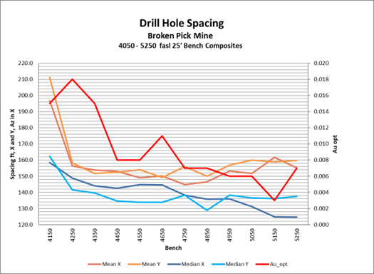
The Hole Spacer 2d graph above is conveniently limited to the pit bottom and the uppermost bench with consequential tonnage. The inputs to DIE for this project can thus be picked for the 4150 and 5250 benches.
DIF = ((160/125) + (160/135)) / 2 = 1.2
GF = (0.015/0.006) = 2.5
DIE = DIF * GF = 3.1
Since the ultimate pit bottom will be pulled relatively deeper by an optimization routine if there is high-grade at depth, there is risk in estimating high-grade here with wide drill spacing. This could be partially addressed by resource classification which might flag resource blocks as Inferred resource at some drill spacing threshold. But that didn’t happen in the case above. The way resource classification is assigned by Estimation Best Practices is by confidence (before reasonable prospect for economic extraction are applied); i.e., factors related to DIF are the only ones taken into account. If the blocks in the model satisfy the modeler’s criteria for Measured or Indicated such as number of holes, nearest or average distance, or variogram range, they pass muster. But in our Case 1a, even though DIF is modest (1.2), the GF amplifies the risk for this project because any estimation error of the higher-grade deep material is very consequential to the shape, depth and size of the ultimate pit. I propose that we designate DIE >= 3 as a benchmark for high resource risk.
Case 1b (below) is a deposit variant that also shows high risk based on DIE. This is a near-vertical-plunging mineralized zone on the margin of a porphyry drilled at depth with progressively more steeply inclined holes from the surface.
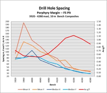
Although the grade in fact decreases somewhat at depth, drill spacing increases dramatically, yielding a calculated of DIE factor of 3.0. The FS pit, optimized on Indicated resource, thus has a significant degree of risk. I’m not suggesting that in this case we see a fatal flaw because of one statistic, but it is can be useful to use some sort of yardstick like DIE to replace or support more subjective opinion and adjectives.
Contrast Cases 1 with Case 2, a gently plunging high-sulfidation epithermal gold manto tested on a fairly regular grid.
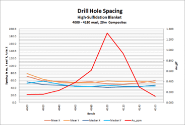
We calculate DIE as follows:
DIF = ((56/52) + (48/46)) / 2 = 1.06
GF = (0.15/0.12) = 1.25
DIE = DIF * GF = 1.3
Due to the high angle of intersection possible with this deposit, there is little decay in drill spacing by bench. The highest grade does not occur at the bottom bench, thus the DIE factor implies more risk than warranted by the nature of the deposit. Still, at a value of 1.3, DIE for Case 2 shows low risk, and compares very favorably against Case 1.
Case 3, a disseminated near-surface blanket returns a DIE factor similar to Case 1, the risky project, but there is a wrinkle to it.
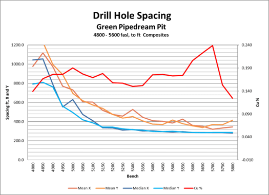
The DIE factor is calculated as follows:
DIF = ((1045/280) + (792/286)) / 2 = 3.25
GF = (0.139/0.124) = 1.12
DIE = DIF * GF = 3.6
If a different endpoint for the pit bottom were picked, the DIF factor would be much smaller since the decay in drill density at depth is not linear. Choosing the 5150 as the bottom bench will return a low value for the DIE factor (1.7) and a lower perception of project risk. In fact, the optimized pit for reporting extended below 4800 bench, the lowest extent represented on the graph because the PEA included Inferred resources. Thus, although this project could have a low-to-moderate DIE factor if optimization were limited to the better-drilled benches, this resource as-presented merits the high DIE factor generated and should be perceived as high-risk.
What about intermediate risk cases? The first graph shown in this post has a DIE factor of 2.4 for the 3450 – 4030 benches, the benches with significant tonnage – not great but not an ‘actionable failure’ either.
Like any tool, one needs to apply the CSF – common sense factor. The geologists might have drilled the liven heck out of the top of the deposit to get an idea of early mine life performance, and just did a government job on the rest. For example, a company does a PEA and a consultant recommends doing a tighter grid in a key area to validate the block model and/or test a grade control assumption. For a pittable deposit, this is likely a shallow zone to be mined in the first years. This will cause the drill spacing curve slope to go more strongly negative depending on the size of the program. In this case, even though the DIF component of DIE, apologies for all the acronyms, looks really bad, the information overall may be perfectly adequate for the classification assigned. We have other tools to assess what the maximum drill spacing should be for the deposit. Thus, we might want to remove the extra drilling program and calculate DIE without it because we didn’t increase the risk by more drilling, we decreased it. I think generally programs like that are rare, or so limited that they won’t affect the overall spacing assessment much. But it’s important to define the problem, limit the universe, and understand the result when calculating any statistic.
I think the DIE factor concept fills a gap in risk assessment that is straightforward and quantifiable, and it is an improvement over relying solely on resource classification for assessing risk. Let’s start with these simple rules, subject to review, analysis and comment due each individual deposit:
- 1 = good
- 2 = pass
- 3 = Fail.
As the database builds for various deposits (I have ~30 in my database) these factors may be modified. One refinement could be to use the slope of regression on the spacing graphs to define the factors, instead of simply picking endpoints as I have done. In the application of any tool, I recommend the application of common sense above all.
Reference
Micheaux, Simon, 2021, Assessment of the Extra Capacity Required of Alternative Energy Electrical Power Systems to Completely Replace Fossil Fuels, Geol. Survey Finland, Rpt No. 42/2021