Practically SG—Bulk Density for Mineral Resource Estimates

This is going to be a really boring read for any but the most habitual miners in the miniscule audience. Even if most of us economic geologist types will agree that rock bulk density is a neglected subject in all facets of exploration, mineral resource estimation and mine production estimates.  It’s one of the three multipliers, the others being volume and grade, for guessing the metal content of a deposit, so what else can you say about it?  Well, if you can assure yourself that you know the difference between specific gravity and dry bulk density and all the parameters that should be included in the calculation of the latter, and if you know how and how not to use tonnage factors, then skip ahead to the next post.  I think you might be in the minority.  For the patient, I hope I can lay out enough detail to help you design, equip, and run a program of bulk density measurement.

Based on my own experience, I’m guessing that the reader hasn’t personally had to conceive, design, set up, supervise, and process more than a few bulk density programs in his/her career. Unless you are an addicted project geologist it just doesn’t come up that often, and as our careers progress from grunt to management, we intersect with this task on relatively few occasions. At the risk of burying the lead, there are several possible forks in designing a program depending on deposit complexity, the condition of the core (broken or porous), the metallic elements present, and geological controls such as lithology and alteration. We can derive bulk density from a series of measured weights, or we can use a combination of measured weights and measured volumes, each method requiring some different equipment and setups. We as an industry could prescribe methods for each condition, but you live in the “free” West so you are on your own. Except for this post, which I hope will help you navigate the possibilities with some logic and prescriptive steps with references to explore for more background.

Background

Probably I was first introduced to the subject in my college mineralogy class through the heavily abridged and updated Dana’s Manual of Mineralogy, 18^th edition (1976),  which correctly defines the term Specific Gravity as the relative density and proceeds through several pages of discussion about how to determine it for minerals and powders.  Fair enough, it’s a text about mineralogy.  Rutley (1926, Elements of Mineralogy) does a great job of explaining and illustrating several methods of determining specific gravity of minerals with instructions which demonstrate a practical knowledge of the subject.  He is of the opinion that the dependence of a specimen’s weight in water on the water temperature can be ignored. Ries and Watson (1936, Engineering Geology) give only a partial and not very adequate definition of specific gravity (“The specific gravity (density) of a mineral is its weight compared with that of an equal volume of water”), and for its measurement: “The time required for the whole determination on this (Jolly) balance should not exceed several minutes.”  I guess that means maybe 3 – 10 minutes, or maybe it depends on the country?  From this I can visualize a Geological Engineer standing over me with a stopwatch while I try to make my measurement quota.  No time for any QA/QC I guess, huh?       

Peele (1941, Mining Engineers’ Handbook, 3^rd ed., Table 10-A-1) explains that specific gravity is dimensionless, whereas density is expressed in terms of mass/volume and is necessary to derive tonnage.  That’s a start for the nuts-and-bolts approach to the use of density in mining.  Palache et al. (1944, The System of Mineralogy of James Dwight Dana and Edward Salisbury Dana) nails the definition of specific gravity as “the density compared to water at 4^o C”, and that it is a constant, but it is, of course, only mentioned in the context of the physical properties of minerals.   McKinstry (Mining Geology, 1948, p. 60-61) jumps right into how to plug in “specific gravity” or tonnage factor to convert volumes to tons but doesn’t explain or use terms with the same precision as more modern texts. 

Consulting my library of economic geology textbooks, Emmons (1918, The Principles of Economic Geology) is wholly concerned with the description and classification of orebodies.  W. Lindgren (1933, Mineral Deposits) skips over the topic despite including other nice weights and measures tables.   For more modern references to bulk density, I looked at my college textbook by Park and MacDiarmid (1970, Ore Deposits), and three others, Guilbert and Park (1986, The Geology of Ore Deposits), Evans, A. (1993, Ore Geology and Industrial Minerals) and Erickson et al. (1992, Applied Mining Geology: General Studies….etc.)  It’s not part of the discussion.  Economic geology, as taught in most universities when I went to school, did not impart a practical knowledge of the appropriate measurement and practical use of density in estimation of “ore”.   One learned a lot about the genesis of ore deposits in the courses but little about how to mine them—you know, the “economic” part of Economic Geology. 

The mundanities of ore deposit exploration and mineral resource estimation, as simple as they are, must be learned from reading published articles on the subject and from practical, hands-on experience with selecting representative samples, and taking measurements oneself.  There are a few papers that are a great help for explaining terms and suggesting ways to measure or apply bulk density.  No one of these papers gives the reader all the information needed to obtain and correctly use bulk density information for different deposit types, sample types, and systems of measurement (e.g., metric and USCS).   A short list can be found here:

Absalov, M. Z., 2013, Measuring and modelling of dry bulk rock density for mineral resource estimation, Applied Earth Sci. v. 122, no. 1, 29 p.

Arseneau, G., 2015, Estimating bulk density for mineral resource reporting, SRK News Issue #51, 2015

CIM Council, 2018, CIM mineral exploration best practice guidelines, Canadian Institute of Mining, Metallurgy and Petroleum, 16 p.

CIM Council, 2019, CIM estimation of mineral resources & mineral reserves best practice guidelines, Canadian Institute of Mining, Metallurgy and Petroleum, 74 p.

Crawford, K. M., 2013, Determination of bulk density of rock core using standard industry methods, Master’s report, Michigan Technological University, 2013, 209 p.

Eggleston, T., 2020, Density data are important, Mine Technical Services Articles 7 -14.

Lipton, I. T. and Horton, J.A., 2014, Measurement of bulk density for resource estimation – methods, guidelines and quality control, in Mineral Resource and Ore Reserve Estimation, the AusIMM guide to best practice, 2^nd ed., Monograph 30, p. 97 – 108.

Lomberg, K.G., 2021, Density: Bulk in-situ or SG?, Journal of the Southern African Institute of Mining and Metallurgy, vol. 121, no. 9, pp. 469–474

Peterson, C. and Thomas J. L., (1972), Aluminum wire tables, US Dept of Commerce, National Bureau of Standards Handbook 109, 58 p.

Scogings, A., 2015, Bulk density: neglected but essential, Industrial Minerals, April 2015

Scogings, A., 2015, Bulk density of industrial minerals: Reporting in accordance with the 2007 SME Guide, Mining Engineering, July 2015, 10 p.

SME, 2014, The SME guide for reporting exploration results, mineral resources, and mineral reserves, Resources and reserves committee of the Society For Mining, Metallurgy, And Exploration, Inc., 65 p.

Smee, B. W., Bloom, L., Arne, D., and Heberlein, D., 2024, Practical applications of quality assurance and quality control in mineral exploration, resource estimation and mining programmes: a review of recommended international practices, Geochemistry: Exploration, Environment, Analysis, vol. 24, p. 1-21.

Lab Protocols Reviewed: Acme, ActLabs, ALS, Dawson, Inspectorate, Metcon, MSALABS, SGS Lakefield, SGS Philippines

As Crawford (2013) points out, existing A.S.T.M. standards are not fully applicable or oriented toward measurement of bulk density from drill core. The published papers omit discussion of historical methods or alternative measurement systems used in different countries, both of which can be valuable.  I am going to try to help the reader sort this out in the sections below.  The Lipton and Horton (2014) article appears to be sanctioned by AusIMM and recommended by CIM, but I think it is not apparently intended as a practical guide for metals exploration.  The authors discuss several methods that no one on this side of the pond with a deadline to meet would ever use.  For example, it describes two variations of a method using water displacement (Water displacement methods 1 and 2) that I’ve only seen in use by a large commercial lab branch in the Philippines. A bucket is filled to the brim, one waits until it stops dripping, then lowers a sample into it collecting the overflow water in another small, pre-weighed dry bucket. The dry bulk density is determined in a 12-step procedure using the six measured weights. As a sort of footnote to the same Lipton and Horton procedure, a “variant” of method 1 is described whereby the displaced water volume is measured from the marks on a graduated cylinder (“beaker”). In my experience, this “variant” is in more common use by some labs (e.g., Inspectorate) and properties I have visited, if nothing else for its relative simplicity.

I can recommend the papers by Crawford and Absalov, and the white papers by Eggleston as the references most aligned to common practice, and the basis of a good start for someone wishing to implement a bulk density measurement program in non-ferrous hard rock deposits.  That is the focus of this paper; discussion of methods for saprolite and unconsolidated materials can be found in other papers in the list.  Frankly, I don’t have any experience with these to share.

Terms of Reference

Density is often confused with specific gravity (SG) which is a unitless ratio of the mass of a sample in air versus the mass of a sample in water. More specifically, the specific gravity is a number that expresses the ratio between the weight of a substance in air and the weight of an equal volume of water at 4° C (Hurlbut, 1971). Thus, if one chooses to refer to “SG” measurements with respect to tonnage calculations there is an implicit assumption that the density of the water used in the measurement was 1.00 gm/cm³.  However, keep in mind that calculations of tonnage in hard-rock mining are made by applying either density,  or tonnage factor (TF), not the dimensionless constant, SG. We therefore implicitly or explicitly take account of water density in our measurements and calculations and use of the term “SG” is an abuse of language of which I myself have been guilty in the past. 

For non-ferrous metal deposits and some others, we measure individual rock density after drying, which should account for pore space, open fractures and variable mineralogy within a specimen, but we extrapolate our density measurements to larger volumes of sometimes heterogeneous materials, thus, bulk density (BD) is commonly what we deal with in mining.  And in the base and precious metals part of the business, we are speaking of dry BD (or dry TF) where water in connected pore spaces and fractures has been eliminated by drying before measurement (exception iron mines which may use in situ bulk density).  Mining engineers and metallurgists deal with both dry and in situ (“wet”) bulk densities in the process streams but we always end up reconciling production on a dry basis since that’s how assays are reported upstream.

Parrish (1993) stated that the most common error found when doing resource/reserve audits is an error in the tonnage factor (more discussion later) used to derive the tonnage of the ore in question. The tonnage factor is directly related to the bulk density of the ore as described by the following equation:

1.0 g/cm³ ≈ 32.0373 ft³/st = 0.0312 st/ft³

The problem is that the density multiplied by the volume yields the tonnage of material; a discrepancy in the density of 10% produces a discrepancy in the metal content of 10%.  Lots of attention is given to metal grade estimates which are supported by extensive statistical analysis, including spatial statistics, metal removal analysis, and domaining.  We tend to treat bulk density as casually, or negligently, as a physician codes a Covid vaccine injury.  The most recent paper in the list above by Smee et al. (2024) also reminds us that QA/QC of bulk density sample measurements is an integral part of any exploration, resource estimation and mining program.

Bulk Density Sampling Considerations

Generally, the number of assays is much greater than the number of bulk density measurements, as pointed out by Parrish and echoed by later authors.  Statistical treatment of the data as presented in technical reports mostly varies from none to minimal in the author’s experience.  Authors Arseneau, and especially, Lomberg have compiled interesting statistics on what percentages of BD data are collected and how they are used from reviews of Technical Reports. It’s not a very impressive performance industry-wide and many of us have recognized this in their own experience over the last decades.  Eggleston, in his discussion of density sampling, provides some good considerations in selecting the number of samples needed for adequate density estimates, and discusses the considerations and limitations in taking representative samples.  I agree with his statement: “Many projects collect a density sample on either side of each lithological change and at specified distances down holes (5 m or 10 m is common). This procedure will generally generate sufficient data to adequately estimate the densities for each ore and waste type.” To that statement,  I’ll add that alteration or mineralization boundaries may also trigger a measurement for certain deposits.

As with any sampling we do, more is better, and systematic is better than left to discretion.  Why aren’t standards prescriptive in this aspect?  One should have to prove that he can shortcut specific minimum guidelines set for various types of deposits.  Any negative consequences would be potentially less severe than leaving sampling frequency and methods to the discretion of individual QPs of variable competence and integrity.  The documented historical track record for discretionary application of bulk density data and estimates as documented in technical reports is poor.

We need to understand the bulk density of waste material as well as for ore.  Waste must be mined and handled.  Waste dilution is a modifying factor and is incorporated in Mineral Reserves by modern definitions.  Thus, if we are mining a vein, we need to take some samples of the “bulk waste” that must be crossed in the development.  We need systematic sampling of any material to be taken as dilution waste, and the ore.  If the deposit is a disseminated, bulk-mineable type, systematic sampling is appropriate throughout the explored rock mass.

Following are some guidelines about how to choose samples of drill core, assuming you don’t know much about mineralization controls at the outset of a project:

• Choose a sample spacing that will allow at least a nearest-neighbor estimate for multiple BD domains; e.g., every 15 or 20m down the hole — particularly critical for a first resource estimate
• Samples will be selected by individual core loggers while the core is being logged—if more than one piece is selected in a contiguous interval one is implicitly assuming that there is no void or core loss between the pieces
• Samples are marked in the core box and removed after logging and photographing, leaving a block to mark the location.  They are returned to the core box after BD measurement.
• Generally, samples are whole core, generally 10 – 20 cm long ( ~ equal support), or rock samples of equivalent size, washed to remove any sand or grease on the surface
• Sawn core halves can be used for BD measurements when no other sample is available and/or where wax coating is required — where possible measure BD before sawing and return the sample to the box (see discussion of alternate wax coating method in later section)
• Sample spacing is adjusted to honor and break on one, or all of rock type, alteration, mineralization type
• For extremely crushed core or gouge, if recovery is determined to be near 100%, sample the entire interval, or if impractical due to length of run, skip the interval
• For base metal deposits where density is likely to be estimated based on certain metal assays, the density measurement ‘From – To’ should be the same as chosen for the assay; i.e., all core in an assay interval must be selected and measured so that the assay attributed to the interval density is representative—the core is returned to the box after measurement and assigned a tag in sequence as part of the assay sampling procedure
• Sample From-To, geology and physical characteristics are logged to fields contained in a separate BD table indexed to the drill hole ID

With respect to the last two points, a measurement apparatus must be designed to have the capacity for longer intervals; e.g., a larger bucket and a larger weighing pan (see discussion in Equipment Needed, below).  This extra accommodation might not be practical or necessary for projects with generally competent ground.

When I was working in Russia in the early 2000s, they had the prescriptive methods down.  For the open pit part of the deposit, two pits were excavated—I’m remembering something like 3m x 3m — with jackhammers in the wide gold vein at different locations.  First, the surface was washed and surveyed in excruciating detail.  All the material taken from the excavation (blasted or dug) was collected on a tarp, dried and weighed.  The surveyors returned to survey the excavations and calculated the excavation volume.   Simply, Mass/Volume= Dry Bulk Density (BD).  The density thus equated as closely as possible to a true bulk density of that material.  The procedure was repeated underground at two locations to represent the deeper mineralization.  In this case, a canvas was placed on the sill.  After surveying and then blasting, the material on the canvas was collected, dried and weighed, followed by another detailed survey.  These densities were applied to the entire deposit with an implicit assumption that the few measurements were representative of the deposit.  Ok, maybe that’s a stretch.  Interestingly, the method was not unknown in the West a century ago.  McKinstry (1948) gives a general outline of a variant of the method where the excavations are filled with known volumes of sand, shot, grain (!) or other material, or by making a plaster cast of the excavation, coating it with paraffin, and then measuring the water displacement.  He notes that enough measurements must be made to ensure that they represent the deposit.  The excavated volume method for BD seems to be discarded by “modern” Western authors. 

Granted, there are concerns about the former (?) Russian method with respect to representativeness, but who can argue that they aren’t good samples?  We should know that we will tend to underestimate BD due to selection bias to some extent in our avoidance of broken and/or crush zones and voids.  Why wouldn’t we perform some QA/QC on our beloved core measurements with this direct weight/volume measurement technique?  And there are instances where the QP has factored densities down based on a judgment that a representative sample of the rock mass from core is impossible in broken ground.

Equipping for Bulk Density

If you want accurate and precise bulk density measurements, do them yourself.  Last I checked, no commercial lab has a thorough protocol or returns any QA/QC information, and I reviewed several assay and metallurgical laboratories in my survey.  It’s a sidelight for them.  

Hopefully, your project has a core shack that has a dedicated and temperature-controlled space at least 3 m x 4 m in size that is equipped as follows:

• Fresh and de-ionized water supplies
• Good lighting
• Networked computer workstation
• Sturdy vibration-dampened bench
• Triple-beam (up to 2.5kg with 0.1g precision) or electronic balance (up to 12 kg with 0.01 or 0.1 precision, as needed)
• Wire or rod, and bucket or basket for suspending sample in water
• Calibration weights
• Sample pans for organizing samples for oven
• Drying oven with timer (can be outside the space reserved for measurements)
• Racks for staging and/or cooling sample pans
• Tongs, wires, brushes for handling and cleaning samples
• Hot plate or wax pot with temperature control that can heat to 57^o C for paraffin coating (Crawford, 2014)
• Graduated cylinder for quick measurements on small samples
• PPE in use and fire extinguisher within reach

For almost all hard rock metal mines the wax-coating procedure should be chosen unless it can be empirically proven that for your project it is not necessary due to lack of porosity and permeability of the core.  In fact, it is not a sufficient method for some rock; e.g., wax coating is not appropriate for samples that have surfaces with large vugs or pitting.  It will be necessary to use a shrink-wrap method, as opposed to vacuum sealing, that will just cover the gaps in the cylindrical form of the core, or a procedure described by Crawford (2013) and summarized in a later section of this post. 

A wax pot can be obtained for ~$50 at any ski shop like the one shown by Crawford (2014) and in this post as Figure 1:

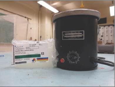
Figure 1 Wax pot with temperature control (from Crawford, 2014)

A Colombian project with pretty competent core saved a chunk of change by substituting a bank of heat lamps (Figure 2) over a steel-topped bench for an expensive drying oven!

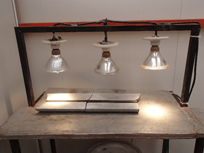
Figure 2  Heat lamp alternative for sample drying

De-ionized water (Type II) and distilled water are available at high prices in retail stores or can be purchased in bulk totes or drums for a third of the retail price (~USD1.50/l).  I advise not stressing too much about the various grades of de-ionization, rather, focusing on availability and price.  What we generally don’t want to use is tap water, and especially, water with lots of dissolved or suspended solids.  If there are signs around the project like this one …

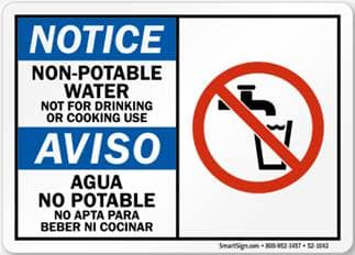
… maybe this is a clue that you need to be looking around for an alternative water supply for immersing samples.

For projects near the North Pole, or overly air-conditioned tropical locales, a heater can be immersed in the bucket of water to provide a constant temperature.  A heater with a readout is not significantly more expensive than a simple thermometer to record the ambient temperature and either choice is fine.

The configuration for weighing typically looks like one of the two scenarios: Suspension below the balance or on top of the balance by use of a supporting stand as shown in Figure 3. 

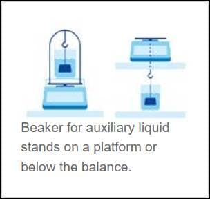
Figure 3 Typical configuration of bulk density measurement (from: https://www.mt.com/us/en/home/applications/Laboratory_weighing/density-measurement.html)

You will need a good stable and vibration-dampened bench and floor with moderated airflow like you see in an assay weighing room (e.g., concrete base), or a compromise setup such as this one offered on a commercial site (Figure 4):

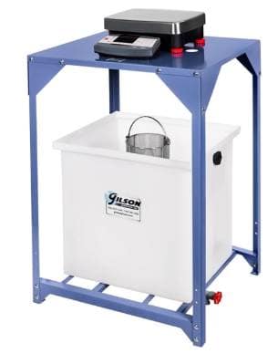
Figure 4 Bulk density bench setup with 30 gallon water tank, balance, and wire basket (https://www.globalgilson.com/specific-gravity-bench)

For this setup, a rod is needed to connect the wire basket to the balance, and you could probably just use a 5-gallon bucket instead of the expensive tub shown.  Some very nice balances customized for density measurements are marketed by vendors such as Mettler-Toledo, Drawell, Shimadzu, Ohaus and others with wide variation in price.   These provide semi-automated calculations and digital export, and will allow input of the liquid density,  But I don’t see one that will include the wax density in the calculation.  You will want to measure to at least 0.1 g precision; some balances, especially digital ones may permit recording to 0.001 g, a precision which is going to be unnecessary and likely not appropriate considering all the factors in the process. 

A relatively indestructible triple-beam balance with an assembly for suspending a weight is shown in Figure 5:

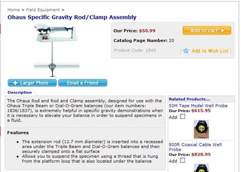
Figure 5. Example of triple-beam balance with assembly for suspended weight

A couple of typical setups for routine bulk density measurements that I have observed are shown in Figure 6:

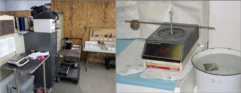
Figure 6. Two examples of bulk density station setups using digital balances

In the picture on the left, the water for immersion is held in the tub below the table.  What I especially like here is that the protocol is printed out and posted in front of the balance.  The setup on the right is very ergonomic with the immersion bucket at the same level as the balance.

For those pesky base metal deposits, a higher capacity digital balance will work better than a triple-beam because a larger length of core can be processed with a single measurement corresponding to an assay interval.  A 20-cm length of HQ-size core with a bulk density of 3.0 g/cm³ will weigh approximately 1.9 kg so the weight of several pieces adds up quickly even if sawn halves are used. The cost of the balance will be substantial if large assay intervals are desired, but aside from extra analytical cost, it is not a problem to assay short intervals that correspond to the density test intervals provided the assay laboratory receives enough mass for its work.  On the Ohaus website many different capacity balances can be reviewed with their specifications.

You’ll probably get calibration weights with the purchase of your balance and those should be sufficient to check your calibration. 

You don’t need the balance to calculate dry bulk density for you.  If you have the raw weights recorded, all calculations can be done in a spreadsheet such as the one copied in Figure 7, or with a scripted database calculation.  The measurements are recorded sequentially from column to column.  They include repeats for each weighing.  The trifling corrections for wax and water density are recorded.  Why ignore them when it’s so easy to build a formula that will accommodate repeated calculations?  I recommend buying paraffin from a vendor who can supply a density for it, and then, why not check it before using it (Hint: It will float so maybe need a graduated cylinder for this)?  The dark gray columns show intermediate calculations and are protected from overwriting.  The bulk density result shown in the yellow column is written if it passes checks based on the recorded measurements.   Otherwise, if checks fail using a 0.25% or 0.5% failure threshold, whichever you set, an appropriate error message is displayed.

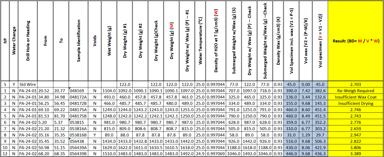
Figure 7 Bulk density data entry and calculation template

Per my previous post, Well-Rounded Estimates, bulk density measurements can generally be reported with 3 – 4 significant figures; however, bulk density block model estimates reporting to more than 3 significant figures stretch credibility.  Also, given that we very likely have some degree of unavoidable sampling high bias with respect to our avoidance of voids and crush zones with poor recovery, we should probably round down, or even truncate the results. Thus, the result in the last column and row of Figure 7 would be reported as 3.38 t/m³ instead of 3.39 t/m³.

The template in Figure 7 can be fleshed out with columns (fields) for metadata like date, sampler’s name, vaccine passport number, drill hole name, drill hole interval, material type code(s) from a picklist(s), descriptive notes and/or comments on the measurement.  The water density column can be populated from a lookup table that references the recorded temperature.

QA/QC for Bulk Density

QA/QC should enter into the estimates of bulk density in a block model.  You don’t have to, and most often shouldn’t use all of the data collected for a project.  If the geologist or technician didn’t achieve constant weights, repeat the measurement or reject it.  There will be outliers in most data sets.  I routinely flag 2SD apparent outliers in the data within any domains or subsets based on lithology, alteration or mineralization that I have determined.  These are reviewed individually because they may represent measurement or recording errors which cause rejection, or may be valid based on the geology controls such as mineralogy, lithology, alteration, or structure and should be included in any average values or interpolation.  A 3d plot with geology context may help with a decision of whether to retain or reject apparent outliers.

For complex, or large data sets, histograms for each potential BD domain or grouping are a good tool to accompany the statistical table. Where there is dependency of BD and metal grade, scatterplots should be reviewed with respect to general correlation and outliers. These can be generated for each metal as part of the Analysis Toolpak multi-element regression tool (see Estimating Block Bulk Density, below).

Smee et al. (2024) recommend including standard reference materials in the measurement procedure. This will help identify other issues that could occur besides an uncalibrated balance. These include dirty water, a strong breeze in the measuring area, or a problem with the down-rod or balance stand, among possible others. For most metal deposits, a clean aluminum wire standard (SG = 2.70; Peterson and Thomas [1972], Table 1) or small bar will serve. But you can always do other checks, too.  Put a U.S. Silver Eagle on the scale and see what you get.  It’s supposed to be 0.999 fine.  If the density is much different than 10.5 g/cm³ you got ripped off by your EBay merchant…or by the U.S. Mint!

Recently, I reviewed a bulk density data table from a large gold project.  The set included two measurements flagged as -2SD outliers with values just over 1.0 g/cm³, obvious errors, and another +2SD measurement >12 g/cm³ where most of the data fell between 2.0 and 3.0 g/cm³.  The latter might be valid if attributable to a massive sulfide of almost pure uraninite with a dash of electrum, but I rejected it because there was no record of the raw data or any notes about the sample. 

Also recently, I was assisting with a new bulk density measurement setup in a core shack for a mine. During a run-through of procedures, the geologist recorded the first weight incorrectly, assigning 2.0 kg. This error was discovered in another training check in which I had the geologists calculate the BD for the specimen. The BD seemed “off”. A second geologist re-weighed the sample and recorded 2.8 kg and the resulting BD looked much more reasonable. The first record was a transcription error. This sort of error is why the template in Figure 7 includes columns for checks of each weighing. Ideally, this is done by processing a group of samples in each step and then re-processing the group in the check step so that there is a time lapse and some physical changes, even a coffee-break, between readings.

All discrepancies should be addressed to the extent possible in real time and the resolution documented in a database field. This field, and fields for the geology codes needed for each sample are not shown in Figure 7 to save space here.

A supervisor or peer should review, as a minimum, the raw data for each group and the BD final results before samples are returned to their boxes or otherwise stored away.

The database manager should arm controls and warning flags within the database recording module used in the core shack and for the project database import process to catch any remaining errors.

All procedures from sample selection, collection, measurement, calculation, QA/QC, storage, and reporting should be incorporated into a written protocol. Put the auditor’s hat on and write it assuming that you will someday ask for the document and check the items off as you go through the project database.

Post a written copy of the relevant portions of the written protocol on a board in the core shack.

The Geology Department should include a heading and section on BD in its periodic QA/QC reports.

Measuring Bulk Density

We have selected our samples per the considerations and procedures discussed above, and they are staged and ready for measurements.  The process for one sample continues in the BD measuring area with steps 4 – 21:

1. Change water for immersion before the first measurement and as needed during measurements.
2. Sample should be carefully cleaned to remove any loose material attached to the core. In most cases, this can be accomplished by placing the sample under running water and gently brushing the core. If drill grease is present, it should be wiped off and degreased thoroughly
3. Tare the balance for the measurements of sample in air
4. Check the balance calibration with one of the calibration weights—results should be within 0.1%
5. Density sample is weighed on an electronic or triple beam balance and the “received” mass recorded in a spreadsheet to the nearest 0.1 g or 0.01 g
6. Sample should be dried for a property-specific, empirically derived time at a temperature of <100^oC  to ensure that all water has been removed from pores in the sample (~4 – 12 hours)
7. Remove the sample from the oven and allow it to cool to ambient temperature (~ 1 – 2 hours)
8. Sample is weighed on an electronic balance and the “Dry Wt #1” mass recorded in a spreadsheet
9. Return sample to the oven for an additional 1 – 2 hours of drying
10. Sample is weighed on an electronic balance and the “Dry Wt #2” mass recorded in a spreadsheet
11. If Dry Wt #1 – Dry Wt #2/(Dry Wt #1 – Dry Wt #2/2) >= 0.1%, then the sample should be returned to the drying oven, weighing process repeated and the Dry Wt #2 and #3 compared
12. If no paraffin coating or shrink wrap is used, go to step 16
13. Using tongs, or two loops of thin wire to hold the specimen, quickly dip it in the melted paraffin, remove after a couple of seconds, and allow the paraffin a short time to harden
14. Weigh the coated sample and record the weight as Dry Wt+Wax
15. Tare the balance with the wire basket suspended in the water container
16. Place the samples, fully immersed, in the wire basket—if any water bubbles adhere to the sample, use a light bottle brush to remove them
17. Weigh the sample suspended in the basket in water; record the immersed sample weight as Wt in Water+Wax, or if no coating is applied simply record as Wt in Water and skip step 18
18. Remove the sample and air dry (can assist with preliminary towel-dry), then check the dry weight to ensure that no water was absorbed by the sample in the immersion process

I believe the discussion and numbered steps above are a starting point for someone to design a protocol for a specific project.  It covers safety, housekeeping, tools, data collection, measurement precision, quality control, and the most common water displacement method for drill core. 

An alternative and reduced workflow will be necessary for the water displacement method using a graduated cylinder. The first 14 steps above are the same though.

Each project/mine will have its own minor procedural variations—it’s the Western way.  Data processing is covered in the next heading. 

Calculating Dry Bulk Density

Depending on your point of view, it’s either frustrating or amusing collecting bulk density formulas.  The simplest calculation is from measurements taking by weighing the sample dry and then dividing the weight by the volume of water displaced by the sample in a graduated cylinder. It’s a bit more involved with wax coating because the volume of wax must be considered, but it can be derived from the difference in weight between the uncoated and coated sample and the known density of the wax.

I’ve presented a procedure above for collecting the data suitable for determination of bulk density by the Archimedes principle along the lines of Absalov (2013, equation 4) and the Lipton and Horton (2014) methods 3 and 4.  One can  calculate the bulk density from the measurements the easy way or the hard way since, remember, we have no specific industry or best practice standards.  The easy way for samples prepared by simple drying can be done using equation (1):

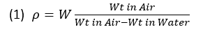
The equation above ignores both the density of water and the density of air, the former varying by temperature, and the latter by elevation and barometric pressure.  If we add these in, the equation looks like equation 2:

Charts are readily available for attaining the appropriate water and air densities using the ambient temperature measurements taken during the measuring procedure.  I doubt anyone considers the air term because it contributes only approximately 0.1% correction to the density of water, which is itself a minor correction (e.g., <1%) to the density derived simply from the weights in the  1^st term of the equations.  At least Lomberg (2021) mentions it and an air density chart can be found at this site: Density of air. The formulas proposed below ignore air, but include water density.

Formulas get a bit more complicated when the wax-coating method is used.  Following is the format in which one would enter the measured quantities in a spreadsheet:

3.  Apparent Dry Bulk Density (BD) = Dry Wt #2/(((Dry Wt+Wax – Wt in Water+Wax)/Water density ) – ((Dry Wt+Wax – Dry Wt #2)/Wax density))

Equation 3 is equivalent to Absalov’s (2013) equation (4).  For uncoated or unwrapped specimens, the spreadsheet formula boils down to simply:

4. Apparent Dry Bulk Density (BD) = (Dry Wt #2/(Dry Wt #2 – Wt in Water)) *Water density

If one records the data in a variation of the template shown in Figure 6, these formulas are easily populated. 

Interval Compositing and Bulk Density

Does your mining software have a box to check for weighting variables as part of the drill hole or channel sampling compositing procedure?  If intervals with different densities are composited for grade, the metal grade(s) will be wrong unless the compositing uses double-weighting by length and density.  Unless there are no density variations within the compositing string between breaks, the default method should be double-weighting when compositing assays. 

Let’s take the example of a stratabound, disseminated gold deposit where each formation has an assigned density based on the QP’s analysis of BD controls.  The composites will be broken on formation contacts.  No density weighting is required in this case because each component assay of each composite has the same density.

But what if we have stratabound massive sulfide deposit where grade and density have mutual dependency according to our analysis? In this case, double-weighting of assays by length and the predicted BD of each assay is required to get correct composite grade.

Finally, a simple example is a string of chip samples in an underground heading.  Ore and waste each have unique assigned densities.  If there is any internal waste to be included in the composites, e.g., a composite taken across the vein or on some regular length,  double-weighting will be required to calculate grade correctly.  For more on this, see my post Correct Estimates of Development Tons and Grade.

Practically, the examples illustrate that in most cases, each assay should have an assigned or calculated BD according to the supporting analysis of the data done beforehand.

Estimating Block Bulk Density

Densities are in many cases applied globally, by a rock type, or by an oxidation type, but bulk density may show some very interesting correlations to metal grades and/or mineral species.  Density is sometimes applied by estimation domains that are constructed from data for the metal(s) of interest.  These domains may not be optimal domains for density assignment and it may be appropriate to have distinct domains for bulk density.  If there is enough data, bulk density can be assigned by interpolation or nearest-neighbor methods.

If mean values are used for bulk density domains, they should be re-calculated after elimination of the outliers, discussed in the section QA/QC for Bulk Density, above.  I have reviewed resource reports by QPs who use the median values for domains instead of the mean.  I think one should justify the use of the median for this purpose instead of the mean because it does not seem to be optimal.

Use of multi-element regressions to assign density is appropriate for most base metal mines and some skarns. Tight regressions may require obtaining sufficient assays of gangue metals such as iron, calcium, magnesium or manganese which might not normally be assayed. If there are more than a couple of dense species in a mineral assemblage, McKinstry (1948) suggests that a stoichiometric approach of allocating assays to individual minerals as percentages might be necessary to produce robust correlations to measured densities.    While it isn’t necessary or in any way feasible to collect as many bulk density samples compared to assays, all density samples need to include analyses of the elements needed to estimate bulk density, and ultimately tonnage.  This, unfortunately, is not universally done.  It’s expensive to add an ICP package for every sample. It is incumbent on the geologist to determine analysis methods and protocols early on in an exploration program that will be sufficient to characterize bulk density and allow extrapolation of bulk density to block models.

Let’s add a bit about the implementation of multi-element regressions.  How do we know we have a useful result from a regression?  I use EXCEL’s Data Analysis Toolpak to plot these.  Let’s say I choose silver, copper, lead, zinc and iron as the element group to evaluate versus measured BD.  I review the statistical output and the data clouds on the graphs. We want to see high correlation coefficients between one or more elements and BD for the model we choose.  Residuals should be reviewed, especially at the extreme ends of the graphs.  Are some outliers causing a bad fit and should they be clipped in a second run?  Which element(s) has a significant P-value (i.e., <0.05), and thus, which elements used in the initial regression can be ignored on a subsequent run?  The final run will use the filtered data and the significant element(s).  The example in Figure 8 is a very simple regression of BD with a mystery metal, “Tb”.

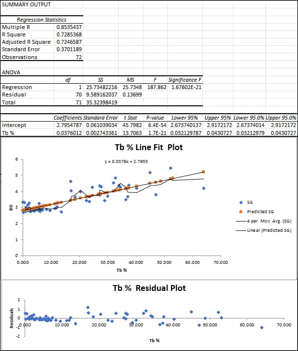
The regression statistics show a reasonably good correlation coefficient (0.85) for BD with Tb%. The scatter and residual plots do not show especially concerning outliers. The equation shown on the scatterplot is made into a database calculation.  After block grade estimation, block density is calculated for each block using the estimated Tb grade.  If we include additional significant elements besides Tb% in the regression, then we will have a separate coefficient for each element. And my final word is that I’m not a statistician, so, dear Reader, feel free to share any comment you may have on this discussion.

Even if bulk density controls are established through experimentation and analysis, often we are stuck with lots of legacy data that may be incomplete with respect to the elements needed to obtain good estimates of bulk density and tonnage.  For example, legacy assays from polymetallic base metal-silver veins in Idaho’s Silver Valley mines may include only lead and/or silver in one type of vein, or copper and/or silver in another.  For the lead-silver veins, an acceptable regression can be obtained using lead or silver assays alone due to the high specific gravity of galena, the dominant mineral, and its silver content.  However, in the copper-silver veins, it is necessary to include iron, copper and silver at least in the regression because there are concentrations of multiple elements with relatively high density.  To adequately characterize the vein halo (dilution) density , a stoichiometric approach might be most robust, requiring additional analysis of Ca, Mn, and Mg which can be allocated to carbonate minerals and pyrite.  But these elements can also be added to a regression matrix to determine if they give good results compared to measured densities.

Another example of a legacy data issue is when a gangue metal becomes a potential pay metal, like antimony.  Antimony is quite the rage at this writing, and several mines and projects are scrambling to take advantage of Federal  grants and loans (the hog trough) to stimulate its production.  Much of the information about antimony contained in the Yellow Pine (Stibnite Project) gold mine and Silver Valley mines in Idaho is from legacy assays and/or mill concentrates produced in the World War II era and/or under DMA and DMEA contracts in place from 1950 to 1958.  In these cases, it may not be possible or feasible to evaluate bulk density of antimony ores accurately because sample material is unavailable from portions of historical deposits.

As mentioned above, there are cases where bulk densities have been factored down in mineral resource estimates due to concerns about the representativeness and/or bias of samples chosen or available for measurement. 

Do we take any consideration of the quality of our bulk density information and estimation into account in our NI 43-101 classification scheme? No, almost nobody does, and I can’t point to any technical report where bulk density uncertainty is an explicit criterion for this.  It’s one of those charming inconsistencies in the mining business and item 6 in the post Trust the Science – Geo Logic, but I will be interested in any cases that readers know of where bulk density is explicitly incorporated in classification.

Density Considerations for Third World Countries

Because my possibly imaginary audience is of North American origin, including the largely de-industrialized U.S. with its own colorful but archaic measurement system, we should include discussion of a variant in bulk density calculations.  The U.S. uses United States Customary System [USCS] units, also referred to loosely as Imperial units which are in most respects, except liquid volumes, identical. In the U.S., we need to address Tonnage Factors (TF).  Most metal mines in the U.S. by tradition have used a Tonnage Factor (TF) to convert in situ rock or stockpile volumes to short tons.   It is an unnecessary and unfortunate choice for a few reasons, unnecessary because a tonnage factor can be converted to a density avoiding calculation problems, discussed below, and unfortunate because it messes everybody up who isn’t well-versed in our archeological industry.  TF is expressed in units of cubic feet per short ton (ft³/st).  TF is the reciprocal of bulk density; thus, to convert a volume of rock to short tons one must divide the volume by the TF, whereas using bulk density, the volume conversion involves multiplying the bulk density and volume.   Another inconvenience is that we generally collect our bulk density (BD) data using metric units such as g/cm³, so to derive the corresponding TF we need to convert the measurements to ft³/st with conversion factors, such as:

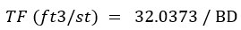
or,

Or, here’s one from Parrish: “cu ft/st = .0.9072 divided by Sp.g. times 0.02832”.  Translated, this reads:

These formulas all give the same result depending on how many keystrokes you want to use to enter and how many significant digits you think are appropriate. 

The dumb part of using TF is that it is a non-additive variable; that is, one cannot average TFs just as you cannot average speeds.  This leads to a common error that is committed in many U.S. mines, projects and consultancies.  We collect density data, convert it to TF, and then average the TF measurements, perhaps then converting the average to get a mean TF.  That will return an incorrect result. To properly use TF in a calculation using U.S. customary units (e.g., cubic feet and short tons), it must be converted to the equivalent density in these units.  For example, a tonnage factor of 1 ft³/short ton is equivalent to a density of 0.1 short tons/ft³.  This density can be multiplied by volume to arrive at tons just as you would do with a metric project.  Density expressed in U.S. customary units or in metric (SI) units is additive and can be averaged.  For example, the average density of a block comprising two equal-size smaller blocks is the simple average of the densities of each of the smaller blocks.  Some mining software packages like Vulcan and Micromine can accommodate either metric or USCS units explicitly or implicitly, but you can’t, or shouldn’t, blend systems inside a specific project. 

Why didn’t we convert all industry measurements to metric way back when our national IQ was still above 100?  Maybe because we are under the delusion that we won WWII and we can do anything we want, even if it’s harder?  Maybe because we have an ideological bent and are miffed at how some of the data supporting the metric system calibration was faked by a French scientist over 200 years ago (reference: Alder, K., The Measure of All Things), notwithstanding that operation within a decimal system is the easiest system of measurement? Regardless, there will always be legacy data for mining properties where density issues may have to be dealt with by conversion.

What happens without prescriptive procedures…

Coatings like shellac, varnish, beeswax, hairspray and food wrap are listed as common sample sealants by Crawford (2013) and Lipton and Horton (2014) to which I’ll add paint (SGS).  I recently ran across a new coating technique for drill core that would be a candidate for some choice names, but we’ll just describe it and leave it at that.  To wit:

• The sample is dried, coated in Vaseline, and then weighed
• The sample is then placed in a graduated, water-filled cylinder
• The amount of water displaced is measured
• The bulk density is then calculated as the weight of the sample divided by the volume of water displaced

Since this was being done at a mine in a South American country with a hot climate, the Vaseline must be imported and may be subject to new tariffs and/or economic sanctions.  But aside from this problem, I just wonder how they manage to keep from getting petroleum jelly on, or in the cylinder, and their hands, and their clothes…

And how do you measure the volume of Vaseline applied?  There’s no correction.  Anyway, this group is  “thinking out of the box (or jar)” and deserves special mention.  If they chose their samples well, they have got better data than a lot of projects that just operate with a few plugged density values, so you can’t be overly critical.   

But in the absence of complete and practical guidelines from our regulators and sages, there arise opportunities for improvement and innovation.  For example, Crawford (2013, Appendix E) describes a method for porous samples comprising an underlayer of shrink wrap and overcoat of paraffin. This method can seal the sample without compromising it for other testing purposes.  With this method, core can be returned to the core box after pealing off the wrap and wax and assayed as part of a larger sample interval if desired.  Bulk density is determined according to a detailed procedure and modified formulas provided by that author.

On one point I don’t agree with the discussion in the Crawford paper concerning the goal of eliminating surface pores from consideration.  In my opinion, the shrink wrap and paraffin coating should mimic the original cylindrical shape of the core and preserve the air-filled void space of any surface vugs.  Some experimentation on my part will be needed to determine whether heat-shrinking or vacuum sealing can provide the best conformance to that cylindrical perimeter.  To modify the procedure so that there is no doubt about large pores, I’ll suggest this procedure which I described in an internal QA/QC guide that I developed more than a decade ago for a major gold mining company:

9a.  Carefully drip melted wax into each natural void, until it is filled evenly to the surface of the core. The temperature of the wax used in this step should be somewhat hotter than that used to seal the samples in the wax-immersion bath so that it will flow well and completely fill voids.  Weigh the sample and record weight as ‘Dry Weight w/Wax — #1’ and ‘N’ in ‘Voids’.

Repeat Steps 9 through 14 as for normal samples (this is the submersion of the sample in hot paraffin was described in steps 16 -21 of this post).

Obviously, this is labor intensive bordering on an arts and crafts project, but if you have a vuggy silica-hosted gold deposit running +2 g/t Au in an open pit mining configuration you can do this without upsetting the slide rule types too much.

Happy BD!

P.S. Thanks to C. Morgan for collaboration on recent program setup which gave me the idea for this post and to Barry Smee for helpful comments and suggestions!